Stat 643 Spring 2010
Assignment 06
Decision Theory
For convenience, let us rewrite the definitions of certain notations here.
A = {a | a is an action}
D = {δ | δ : X → A is a non-randomized decision rule}
D∗ = {φx | ∀x, φx is a probability measure on A}
D∗ = {ψ | ψ is a probability measure on D}
Z
R(θ, δ) =
L(θ, δ(x))dPθ (x)
ZX Z
R(θ, φ) =
L(θ, a)dφx (a)dPθ (x)
Z Z
ZX A
R(θ, δ)dψ(δ) =
R(θ, ψ) =
L(θ, δ(x))dPθ (x)dψ(δ)
D
D
X
S 0 = {yδ = (y1 , . . . , yk ) | yi = R(θi , δ), i = 1, . . . , k}, Θ = {θ1 , . . . , θk }
S = {yψ = {y1 , . . . , yk } | yi = R(θi , ψ), i = 1, . . . , k}
51. Consider Θ = A = {1, 2, . . . , k}. For any given convex subset S ⊂ [0, ∞)k , we are going
to show that there exists a collection of behavioral decision rules D∗ with S as its risk set.
Suppose X has a degenerate probability distribution such that Pθ ({1}) = 1, ∀θ ∈ Θ. Consider
loss function L(θ, a) = |θ − a|, then for any y = (y1 , . . . , yk ) ∈ S, define a behavioral decision
rule φy in the manner that R(i, φy ) = yi , i = 1, . . .P
, k. This is valid, because φy would be
uniquely determined by the set of linear equations ki=1 |θ − i|φy1 ({i}) = yθ , θ = 1, 2, . . . , k.
P
In summary, let D∗ = {φy | y ∈ S, ki=1 |θ − i|φy1 ({i}) = yθ , θ = 1, 2, . . . , k}, then D∗ would
have a risk set as S.
52. Note that X = {0, 1} here.
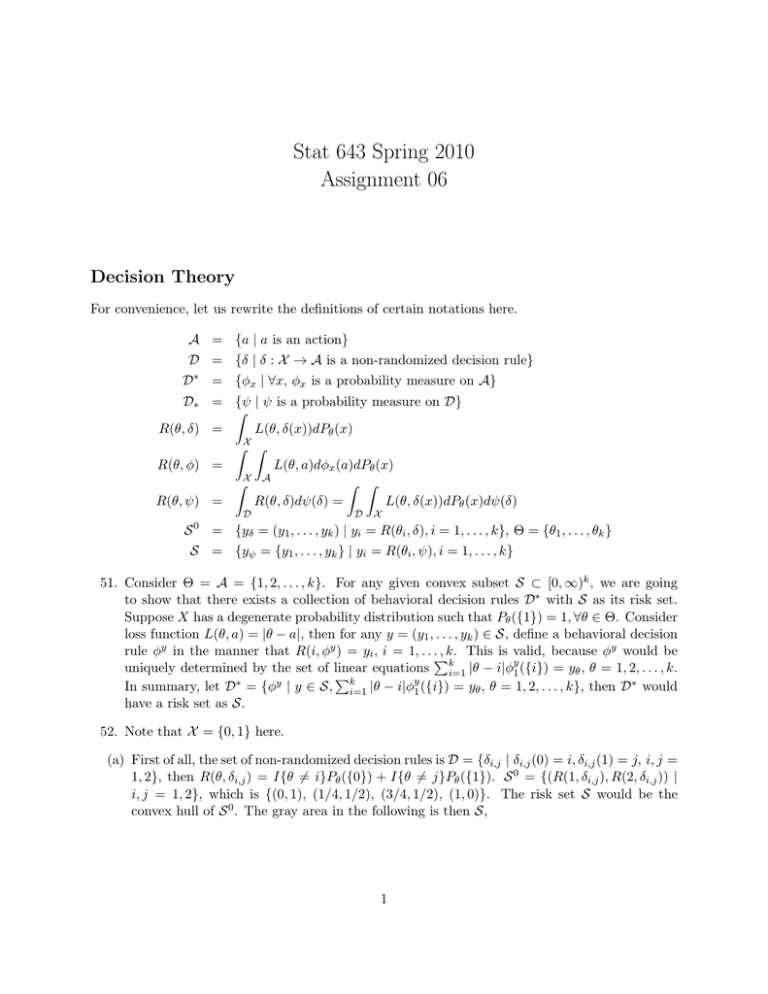
(a) First of all, the set of non-randomized decision rules is D = {δi,j | δi,j (0) = i, δi,j (1) = j, i, j =
1, 2}, then R(θ, δi,j ) = I{θ 6= i}Pθ ({0}) + I{θ 6= j}Pθ ({1}). S 0 = {(R(1, δi,j ), R(2, δi,j )) |
i, j = 1, 2}, which is {(0, 1), (1/4, 1/2), (3/4, 1/2), (1, 0)}. The risk set S would be the
convex hull of S 0 . The gray area in the following is then S,
1
0.0 0.2 0.4 0.6 0.8 1.0
R(2, δ)
0.0
0.2
0.4
0.6
0.8
1.0
R(1, δ)
(b) For any elemental φ ∈ D∗ , the risk function is R(θ, φ) = Pθ ({0})(I{θ 6= 1}φ0 ({1}) + I{θ 6=
2}φ0 ({2})) + Pθ ({1})(I{θ 6= 1}φ1 ({1}) +
PI{θ 6= 2}φ1 ({2})). And for any ψ ∈ D∗ , the
corresponding risk function is R(θ,
Pψ) = i,j∈{1,2} ψ({δi,j }){I{θ 6= δi,j
P(0)}Pθ ({0}) + I{θ 6=
δi,j (1)}Pθ ({1})}, which is Pθ ({0}) i,j∈{1,2} ψ(δi,j )I{θ 6= i} + Pθ ({1}) i,j∈{1,2} ψ(δi,j )I{θ 6=
j}. This actually motivates the correspondence between φ and ψ, which is determined by
φ0 ({i}) = ψ({δi,1 }) + ψ({δi,2 }), φ1 ({j}) = ψ({δ1,j }) + ψ({δ2,j }), i, j = 1, 2. Then for any
ψ ∈ D∗ , we can define φ using the above relationship, and they would have the same risk
function. On the other hand, for any φ ∈ D∗ , we can specify at least one ψ who satisfies
the above relationship and has the same risk function as φ. The easiest way of thinking
about it, in this case, would be thinking about the relationship between joint distribution
and marginal distribution of a 2 × 2 probability table.
(c) All admissible risk vectors would be those points, which is the lower boundary of S, i.e.
λ(S) = {y | Qy ∩ S̄ = {y}}, as indicated by the blue lines in the above figure. Notice further
that A(D∗ ), the admissible rules in D∗ , is complete here by just looking at the above risk
set plot. Thus it is minimum complete.
(d) Note that for each φ ∈ D∗ , R(g, φ) = pR(1, φ) + (1 − p)R(2, φ). Now consider the line
(1 − p)y + px = b. When p = 1, the risk vector corresponding to the Bayes with respect
to g would be (0, 1). For 0 ≤ p ≤ 1, the line becomes y = −p/(1 − p) · x + b/(1 − p).
For simplicity, define L = {(x, y) ∈ R2 | (1 − p)y + px = b, b ∈ R}, then the set of risk
vectors that are Bayes versus g is {(x, y) ∈ S ∩ L | Q(x,y) ∩ (S ∩ L) = {(x, y)}}, where Q(x,y)
is the lower quadrant of (x, y). Then we see that two particular priors, corresponding to
−p/(1 − p) = −2 and −p/(1 − p) = −2/3 have more than one decision rules. In all, when
0 ≤ p < 2/5, then answer is {(1, 0)}; when p = 2/5, the answer is {(λ/4 + (1 − λ), λ/2) |
0 ≤ λ ≤ 1}; when 2/5 < p < 2/3, then answer is {(1/4, 1/2)}; when p = 2/3, the answer is
{(λ/4, λ/2 + (1 − λ)) | 0 ≤ λ ≤ 1}; when 2/3 < p ≤ 1, the answer is {(0, 1)}.
(e) The posterior distribution with respect to g = (1/2, 1/2) is πθ|X=x ({1}) = P1 ({x})/{P1 ({x})+
P2 ({x})}, and the posterior expected loss is E{L(θ, φx )|X = x} = E{φx ({1})I{θ = 2} +
φx ({2})I{θ = 1}|X = x} = {φx ({2})P1 ({x}) + φx ({1})P2 ({x})}/{P1 ({x}) + P2 ({x})}. Thus
the Bayes with respect to g = (1/2, 1/2) is φ∗x ({1}) = I{x 6= 1}. Based on the formula de2
rived in part (b), we know that (R(1, φ∗ ), R(2, φ∗ )) = (1/4, 1/2), which is actually the correct
answer due to our analysis in part (d).
53. The joint probability measure of X = (X1 , X2 ) is Pθ × Pθ = Pθ2 . Then the risk function
corresponding to φ defined in the context of this problem is R(θ, φ) = L(θ, 1)Pθ ({0}) +
Pθ ({1})/2. Therefore,Rits risk vector is (1/8, 3/4). Now let’s consider φ0x ({1})
= I{x1 + x2 ≤
R
1}, then R(1, φ0 ) = φ0x ({2})dP12 (x) = P1 ({1})2 = 1/16, R(2, φ0 ) = φ0x ({1})dP22 (x) =
1 − P2 ({1})2 = 3/4, which means φ0 is better than φ in terms of risk functions. Therefore, φ
is inadmissible.
9
3
For a general behavioral decision rule φ̃, note that R(1, φ̃) = 16
φ̃(0,0) ({2}) + 16
φ̃(0,1) ({2}) +
3
1
16 φ̃(1,0) ({2}) + 16 φ̃(1,1) ({2}); R(2, φ̃) = {φ̃(0,0) ({1}) + φ̃(0,1) ({1}) + φ̃(1,0) ({1}) + φ̃(1,1) ({1})}/4.
One can actually solve a equation using φ̃x ({2}) = aI{x1 + x2 = 0} + bI{x1 + x2 = 1} +
cI{x1 + x2 = 2}. This suggests φ̃x ({2}) = 81 I{x1 + x2 = 0} + 78 I{x1 + x2 = 2}. One can
verify that φ̃ here is risk equivalent to φ.
o2
n
= E(p −
54. R(p, δ1 ) = E(p − X/n)2 = V ar(X/n) = p(1 − p)/n, R(p, δ2 ) = E p − X/n+1/2
2
X/n)2 /4 + (p − 1/2)2 /4 = p(1 − p)/(4n) + (p − 1/2)2 /4, and R(p, ψ) = R(p, δ1 )ψ({δ1 }) +
2 /8. To make a behavioral rule equivalent to
R(p, δ2 )ψ({δ2 }) = 5p(1 − p)/(8n)
R R + (p − 1/2)
2
psi, notice that R(p, φ) = X (0,1) (p − a) dφx (a)dPp (x), the most natural choice would be
R
2
φ
R x ({x/n}) = φx ({(x/n2 + 1/2)/2}) = 1/2. In this way, R(p, φ) = X (p − x/n) dPp (x)/2 +
X (p − (x/n + 1/2)/2) dPp (x)/2 = R(p, ψ).
55. Suppose that φ is inadmissible when the parameter space is Θ, that is, there exists φ0 such
that R(θ, φ0 ) ≤ R(θ, φ), ∀θ = (θ1 , θ2 ) ∈ Θ = Θ1 × Θ2 and the inequality holds strictly for at
least one θ∗ = (θ1∗ , θ2∗ ) ∈ Θ. Then clearly φ0 is better than φ when the parameter space is
Θ1 × {θ2∗ }, which is a contradiction. Therefore, φ is admissible when the parameter space is
Θ.
R R
R R
0,
0
56. For any two behavioral
decision
rules
φ,
φ
L(θ,
a)dφ
(a)dP
(x)
≤
x
θ
X
A
X A L(θ, a)dφx (a)dPθ (x)
R R
R R
is equivalent to X A w(θ)L(θ, a)dφx (a)dPθ (x) ≤ X A w(θ)L(θ, a)dφ0x (a)dPθ (x), for any θ.
This means all inequalities would remain the same when multiplying the loss function by
w(θ) > 0. And this suffices to support the fact that admissibility would not change when
changing loss function in this way.
2
2
57. T0 (X) = I{X̄ > 1/2} + I{X̄ = 1/2}/2, then R(θ,
P T0 ) = E{T0 (X) − θ} = θ + (1 −
2θ)Pθ (X̄ > 1/2) + (1/4 − θ)Pθ (X̄ = 1/2), where
Xi ∼ Binomial(n, θ). Now R(θ, T1 ) =
R(θ, X̄)/2 + R(θ, T0 )/2 = V ar(X̄)/2 + R(θ, T0 )/2 = θ(1 − θ)/(2n) + R(θ, T0 ). And R(θ, T2 ) =
Eθ {(θ − X̄)2 X̄ + (θ − 1/2)2 (1 − X̄)} = (θ − 1/2)2 (1 − θ) + (1 − θ)θ2 /n + Eθ {(X̄ − θ)3 }.
58. T0 is a non-randomized decision rule. By Theorem 2.5 from Shao, we can consider δ1 (X) =
(X̄ + T0 )/2 for T1 and δ2 (X) = X̄ 2 + (1 − X̄)/2 for T2 .
3