Due on Monday, April 4 in TA’s office by 5:00 pm
Problem 1
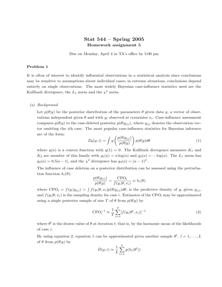
It is often of interest to identify influential observations in a statistical analysis since conclusions may be sensitive to assumptions about individual cases; in extreme situations, conclusions depend entirely on single observations. The most widely Bayesian case-influence statistics used are the
Kullback divergence, the L
1 norm and the χ
2 norm.
(a) Background
Let p ( θ | y ) be the posterior distribution of the parameters θ given data y , a vector of observations independent given θ and with y i observed at covariates x i
. Case-influence assessment compares p ( θ | y ) to the case-deleted posterior p ( θ | y
( i )
), where y
( i ) denotes the observation vector omitting the i th case. The most popular case-influence statistics for Bayesian inference are of the form:
D
θ
( g, i ) =
Z g p ( θ | y
( i )
)
!
p ( θ | y ) dθ p ( θ | y )
(1) where g ( a ) is a convex function with g (1) = 0. The Kullback divergence measures K
1 and
K
2 are member of this family with g
1
( a ) = a log( a ) and g
2
( a ) = − log( a ). The L
1 norm has g
3
( a ) = 0 .
5 | a − 1 | , and the χ
2 divergence has g
4
( a ) = ( a − 1)
2
.
The influence of case deletion on a posterior distribution can be assessed using the perturbation function h i
( θ ): p ( θ | y
( i )
) p ( θ | y )
=
CPO i f ( y i
| θ, x i
)
≡ h i
( θ ) where CPO i
= f ( y i
| y
( i )
) = R f ( y i
| θ, x i
) p ( θ | y
( i )
) dθ , is the predictive density of y i given y
( i )
, and f ( y i
| θ, x i
) is the sampling density for case i . Estimates of the CPO i may be approximated using a single posterior sample of size T of θ from p ( θ | y ) by
CPO
− 1 i
1
≈
T
T
X
[ f ( y i
| θ t
, x i
)]
− 1 t =1
(2) where θ t is the drawn value of θ at iteration t ; that is, by the harmonic mean of the likelihoods of case i .
By using equation 2, equation 1 can be approximated given another sample θ l
, l = 1 , . . . , L of θ from p ( θ | y ) by
ˆ
( g, i ) ≈
1
L
L
X g ( h i
( θ l
)) l =1

(b) Problem
Consider the simple linear regresion model: y i
= β
0
+ β
1 x i
+ i
∼ N(0 , σ and the following dataset i 1 2 3 4 5 6 7 8 9 10 11 x i
15 26 10 9 15 20 18 11 8 20 7 y i
95 71 83 91 102 87 93 100 104 94 113
2
I) i 12 13 14 15 16 17 18 19 20 21 x i
9 10 11 11 10 12 42 17 11 10 y i
96 83 84 102 100 105 57 121 86 100
Assume the following prior distributions:
β i
∼ N(0 , [0 .
0000001]
− 1
) i = 1 , 2
σ
2 ∼ Inv-Gamma(1,0.001).
For each observation:
1) Calculate CPO i
2) Calculate both Kullback divergences.
3) Calculate the L
1 norm divergence.
4) Calculate the χ
2 norm divergence.
5) Interpret the results (i.e. which observations are outliers, and which are influential cases.)
Hint:
This problem can be carried out using WinBugs. You should write one program to do part 1, and another to do parts 2-4.
• In your first program, fit the model and for each iteration t and for each of the 21 observations i compute k i
( θ ) k i
( θ ) =
1 f ( y i
| θ t , x i
)
You may use 6.28 as an approximation for 2 π .
Get the means of your 21 k ’s. These means are CPO
− 1 i need to compute their inverses outside WinBugs defined in equation (2). You will
1 . These inverses will be used as data in your second program. A really useful function inside R is dput . It will write an R object to look like “WinBugs data” format; you have to edit out some of the output though. Run this program to see what dput does:
1 If you wish to get fancy, you may want to use bugs.R inside R (see appendix C of the textbook). bugs.R is loaded on all the 322 Snedecor machines and that will allow you to do all calculations from within R

x<-1:10 x dput(x,"")
• In your second program, with the CPO’s included in your data declaration, you have to compute the different norms. For example to calculate χ
2 divergence, you would compute:
ˆ
( g, i ) =
1
L
X
L l =1
CPO i f ( y i
| θ l , x i
)
− 1
2
Problem 2
Selecting a suitable model from a large class of plausible models is an important problem in statistics. A classic example is the selection of variables in linear regression analysis. One approach to selecting variables is predictive model assessment. This method consists on sampling ”new data” Z from a model fitted to all cases, and seeing how consistent the new data are with the observations.
Thus, comparisons might be made by sampling replicates Z i
( t ) from a normal model with mean µ
( t ) i
, and variance ( σ
2
)
( t ) for each observation at iteration t and then comparing those values with the corresponding y i
.
One comparison criterion is to calculate for each model in consideration the following quantity:
C
2
= n
X
[ { E ( Z i
) − y i
}
2 i =1
+ Var( Z i
)] (3)
Better models will have smaller values of C
2
, or of its square root C . Thus, if for example we have two models: model 1 and model 2, model 1 will be better than model 2 if
C
2
(1)
− C
2
(2)
= n
X
[ { E ( Z
1 i
) − y i
}
2 i =1
− { E ( Z
2 i
) − y i
}
2
] < 0 (4) where C
2
( j ) and Z ji represent the criterion and the replicates obtained under model respectively. Alternatively, model 1 is better than model 2 if C
(1) q
C
2
( j )
.
− C
(2)
< 0 where C j
( j )
( j = 1 , 2) stands for
Our dataset
2 refers to the heat evolved in calories per gram of cement, a metric outcome, for n = 13 cases. The outcome is related to four predictors describing the composition of the cement ingredients.
2
Hald, A. (1952) Statistical Theory with Engineering Applications . New York: Wiley

x
1 x
2 x
3 x
4 y
7 26 6 60 78.5
1 29 15 52 74.3
11 56 8 20 104.3
11 31 8 47 87.6
7 52 6 33 95.9
11 55 9 22 109.2
3 71 17 6 102.7
1 31 22 44 72.5
2 54 18 22 93.1
21 47 4 26 115.9
1 40 23 34 83.8
11 66 9 12 113.3
10 68 8 12 109.4
(a) Using the criterion described in equation 4 evaluate the following models:
Model 1: y i
= α
0
+ α
1 x
1 i
+ α
2 x
2 i
+ α
3 x
4 i
+ ε i
Model 2: y i
= β
0
+ β
1 x
1 i
+ β
2 x
2 i
+ β
3 x
3 i
+ ε
Model 3: y i
= γ
0
+ γ
1 x
1 i
+ γ
2 x
3 i
+ γ
3 x
4 i
+ ε i i
Model 4: y i
= δ
0
+ δ
1 x
1 i
+ δ
2 x
2 i
+ δ
3
Model 5: y i
= φ
0
+ φ
1 x
1 i
+ φ
2 x
2 i
+ ε i x
3 i
+ δ
4 x
4 i
+ ε i
Model 6: y i
= ϕ
0
+ ϕ
1 x
1 i
+ ϕ
2 x
4 i
+ ε i
Model 7: y i
= η
0
+ η
1 x
2 i
+ η
2 x
3 i
+ η
3 x
4 i
+ ε i
Model 8: y i
= κ
0
+ κ
1 x
1 i
+ κ
2 x
3 i
+ ε i where ε ∼ N(0 , σ 2 I).
Use the following prior distributions:
• σ
2 ∼ Inv-gamma(12.5,62.5).
• For the parameters of each model a N(0,[0 .
00001]
− 1 ).
Comments:
• This problem can also be done using WinBugs.
• Two WinBugs functions that may be helpful are the function step() and the function sum() .
The step function takes the following values step( a ) =
( 1 if a ≥ 0
0 otherwise
• A WinBugs example program to obtain draws from the predictive posterior distribution in a simple linear regression model (indicate by the z ’s) is:

model{ for (i in 1:N){ y[i] ~ dnorm(mu[i],tau.y) mu[i] = b[1]+b[2]*x[i] z[i] ~ dnorm(mu[i],tau.y) } for (i in 1:2){b[i] ~ dnorm(0,0.00001)} tau.y ~ ...
}
Data list(y=c(....),N=..)
• If x ∼ Gamma( α, β ), then x
− 1 ∼ Inv-Gamma( α, β ). Both distributions have the same α and β .
Thus, if σ
2 ∼ Gamma(12.5,62.5) then σ
− 2 ∼ Inv-Gamma(12.5,62.5). In the textbook appendix
A (page 580) you will find a description of the relationship between those two distributions.
• The z’s are called “new” since they are realizations from the predictive posterior distribution
(i.e. from p ( z | y )) as opposite to your y ’s that are realizations from p ( y | θ ), where θ stands for all the parameters in your model. Note that your z ’s are what in class and in the textbook are referred as ˜ (see for example pages 8 and 137.) For convenience here they have been called z instead of ˜ , since there is no ambiguity given the fact that the wording of problem
2 assigns the name z to observations drawn from the predictive posterior distribution.
• You have i = 1 , . . . , 13 observations: y i
; and j = 1 , . . . , 8 models, each model with a different mean.
In each iteration, for each one of those 13 observations you draw eight z ji
’s, one for each one of the eight models.
Then, you have to calculate ( z ji
− y i
)
2
, and then you have to sum those values over i for each j . These sums are proportional to C
2 j
. Note that you dont need to consider the part that involves the sum of the variances of the z ij
’s since it will cancel out when you subtract the C 2 from one model with the C
2 from another since all models have the same variance. Further, note that since at each iteration you have only one value of z ij lieu of E( Z ij
).
you have to use this value in
• It may also pay off to be a little inefficient while programming, in the sense that you have to define the mean of 8 different models and they have a different number of parameters (some have three, anothers four, one with five). Thus, you have two choices, one is to define several different loops depending how many parameters your model has. The other is to define an
8x5 matrix where each row will contain the parameters needed to define the mean of each one of the 8 models. This has the advantage that you will need only two double-loops, one for defining the means and another to assign priors. Using this approach you are defining more parameters than you really need, and because of this your code will be inefficient. For this problem however, in terms of machine-time you will expend about an extra nano-second per iteration. Remember, the shorter your program, the easiest to find where the errors are.