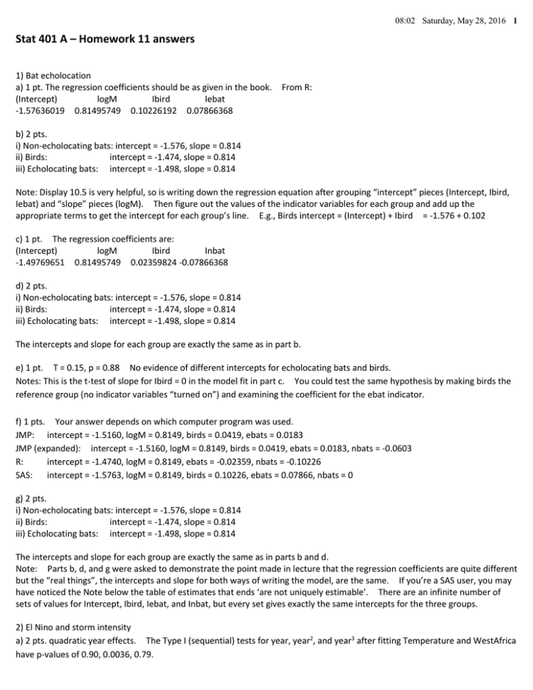
08:02 Saturday, May 28, 2016 1
Stat 401 A – Homework 11 answers
1) Bat echolocation
a) 1 pt. The regression coefficients should be as given in the book.
(Intercept)
logM
Ibird
Iebat
-1.57636019 0.81495749 0.10226192 0.07866368
From R:
b) 2 pts.
i) Non-echolocating bats: intercept = -1.576, slope = 0.814
ii) Birds:
intercept = -1.474, slope = 0.814
iii) Echolocating bats: intercept = -1.498, slope = 0.814
Note: Display 10.5 is very helpful, so is writing down the regression equation after grouping “intercept” pieces (Intercept, Ibird,
Iebat) and “slope” pieces (logM). Then figure out the values of the indicator variables for each group and add up the
appropriate terms to get the intercept for each group’s line. E.g., Birds intercept = (Intercept) + Ibird = -1.576 + 0.102
c) 1 pt. The regression coefficients are:
(Intercept)
logM
Ibird
Inbat
-1.49769651 0.81495749 0.02359824 -0.07866368
d) 2 pts.
i) Non-echolocating bats: intercept = -1.576, slope = 0.814
ii) Birds:
intercept = -1.474, slope = 0.814
iii) Echolocating bats: intercept = -1.498, slope = 0.814
The intercepts and slope for each group are exactly the same as in part b.
e) 1 pt. T = 0.15, p = 0.88 No evidence of different intercepts for echolocating bats and birds.
Notes: This is the t-test of slope for Ibird = 0 in the model fit in part c. You could test the same hypothesis by making birds the
reference group (no indicator variables “turned on”) and examining the coefficient for the ebat indicator.
f) 1 pts. Your answer depends on which computer program was used.
JMP: intercept = -1.5160, logM = 0.8149, birds = 0.0419, ebats = 0.0183
JMP (expanded): intercept = -1.5160, logM = 0.8149, birds = 0.0419, ebats = 0.0183, nbats = -0.0603
R:
intercept = -1.4740, logM = 0.8149, ebats = -0.02359, nbats = -0.10226
SAS:
intercept = -1.5763, logM = 0.8149, birds = 0.10226, ebats = 0.07866, nbats = 0
g) 2 pts.
i) Non-echolocating bats: intercept = -1.576, slope = 0.814
ii) Birds:
intercept = -1.474, slope = 0.814
iii) Echolocating bats: intercept = -1.498, slope = 0.814
The intercepts and slope for each group are exactly the same as in parts b and d.
Note: Parts b, d, and g were asked to demonstrate the point made in lecture that the regression coefficients are quite different
but the “real things”, the intercepts and slope for both ways of writing the model, are the same. If you’re a SAS user, you may
have noticed the Note below the table of estimates that ends ‘are not uniquely estimable’. There are an infinite number of
sets of values for Intercept, Ibird, Iebat, and Inbat, but every set gives exactly the same intercepts for the three groups.
2) El Nino and storm intensity
a) 2 pts. quadratic year effects. The Type I (sequential) tests for year, year2, and year3 after fitting Temperature and WestAfrica
have p-values of 0.90, 0.0036, 0.79.
08:02 Saturday, May 28, 2016 2
Note: The tests associated with these p-values can be interpreted as saying: Adding a quadratic term to a model with Year
significantly improves the fit (p = 0.0036 for year2). Adding a cubic term to a model with Year2 does not significantly improve
the fit (p = 0.79 for year3).
b) 2 pts. Each additional degree of Temperature is associated with a -33.4 unit drop in Storm Intensity, after adjusting for
WestAfrica and Year. A 95% confidence interval for this effect is (-47.7, -19.2). [Or, include the se in the statement of
association, e.g. is associated with a -33.5 (se = 7.1) unit drop.]
Note: I had intended this to be based on the model with WestAfrica and quadratic year (i.e. the result of part a). That was not
explicit. Other numbers based on other models are accepted for full credit, so long as they include an estimate of magnitude
and its precision.
0.00
0.05
d
0.10
0.15
c) 1 pt. No. The largest Cook’s Distance is less than 0.2, which is much less than the concern level of 1.
Note: In case you want see the results, here is the plot:
0
10
20
30
Observation number
40
d) 1 pt. Yes, serious concerns with multicollinearity. The VIF factors for year and year2 are larger than 100000, which
certainly exceeds the concern level of 10.
Note: Some software would not fit the cubic year model. That’s because the correlations between variables are almost 1.
The VIF values for the cubic model exceed 6,000,000,000. Even if software will fit the cubic model, the regression
coefficients are not well estimated.
e) 1 pt. No concerns about multicollinearity after centering (or approximately centering) year.
on how you centered, but they are all less than 2.
The exact VIF values depend
08:02 Saturday, May 28, 2016 3
The plots are:
0
3800000
100
year2
3900000
yearc2
200 300 400
500
600
f) 1 pt.
1950
1960
1970 1980
Year
-10
-20
1990
0
yearc
20
10
There is a very strong linear dependence between Year and Year2 and almost no linear dependence between centered Year and
its square.
Copper and Zinc toxicity.
The plots are:
0.3
3. 2 pts.
Log Protein
-0.2
-20
-0.1
-10
Resid
0.0
0.1
Resid
0
10 20
30
0.2
40
Protein
120
140
160
180
Predicted
200
4.7
I don’t see much to choose between these.
Note: This is not surprising if you plot Protein against log Protein (see next page).
so the plot is nearly linear. That’s why the two residual plots are so similar.
4.8
4.9 5.0 5.1
Predicted
5.2
5.3
The range of Protein values is not very large,
4.7
4.8
logProt
4.9 5.0 5.1
5.2
5.3
08:02 Saturday, May 28, 2016 4
120
140
160
Protein
180
200