MA22S6 Homework 4 Solutions
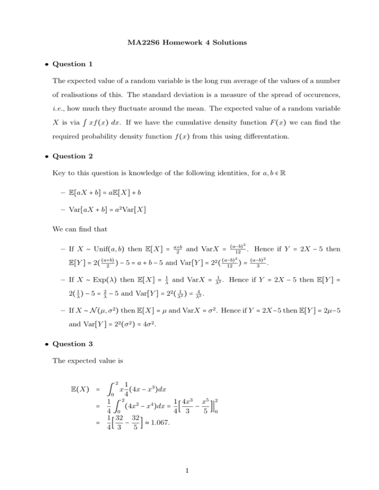
ˆ Question 1
The expected value of a random variable is the long run average of the values of a number
of realisations of this. The standard deviation is a measure of the spread of occurences,
i.e., how much they fluctuate around the mean. The expected value of a random variable
X is via ∫ xf (x) dx. If we have the cumulative density function F (x) we can find the
required probability density function f (x) from this using differentation.
ˆ Question 2
Key to this question is knowledge of the following identities, for a, b ∈ R
– E[aX + b] = aE[X] + b
– Var[aX + b] = a2 Var[X]
We can find that
– If X ∼ Unif(a, b) then E[X] =
a+b
2
and VarX =
(a−b)2
12 .
2 (a−b)
E[Y ] = 2( (a+b)
2 ) − 5 = a + b − 5 and Var[Y ] = 2 ( 12 ) =
2
– If X ∼ Exp(λ) then E[X] =
2( λ1 ) − 5 =
2
λ
1
λ
and VarX =
− 5 and Var[Y ] = 22 ( λ12 ) =
1
λ2 .
Hence if Y = 2X − 5 then
(a−b)2
3 .
Hence if Y = 2X − 5 then E[Y ] =
4
λ2 .
– If X ∼ N (µ, σ 2 ) then E[X] = µ and VarX = σ 2 . Hence if Y = 2X−5 then E[Y ] = 2µ−5
and Var[Y ] = 22 (σ 2 ) = 4σ 2 .
ˆ Question 3
The expected value is
2 1
E(X) = ∫ x (4x − x3 )dx
4
0
1 2
1 4x3 x5 2
2
4
=
(4x
−
x
)dx
=
[
− ]∣
4 ∫0
4 3
5 0
1 32 32
=
[ − ] ≈ 1.067.
4 3
5
1
Calculating E(X 2 ) we see
2
1
E(X 2 ) = ∫ x2 (4x − x3 )dx
4
0
1 2
1 4 x6 2
3
5
=
(4x
−
x
)dx
=
[x − ]∣
4 ∫0
4
6 0
64
1
=
[16 − ] ≈ 1.333.
4
6
Hence the variance is
Var(X) = E(X 2 ) − [E(X)]2
= 1.333 − (1.067)2 = 0.1948.
Taking the square root of this we find the standard deviation of σX = 0.441. Hence on
average a contractor makes $1067. If he made less than $600 in a single job this would
not be hugely surprising, but if he made less than this on average over 2000 jobs we would
be extremely surprised, as this is dramatically less than the long run average. In fact, the
2
sample variance for 2,000 trials would be σX
/2000, hence the standard deviation is then
of the order 0.01, i.e. $10.
ˆ Question 4
The expected value of the exponential distribution is 2, i.e., E(X) = λ1 , giving 2 = λ1 , or
λ = 0.5. This is our rate parameter, used in the cumulative density function X < ≈ =
1 − e−λt . This tells the probability of a wait time less then a specific duration, i.e., the
probability of a wait of less than three minutes is P(X < 3) = 1 − e−0.5×3 = 0.777. By
the memoryless property of the exponential distribution (formally proved in Question 5)
inter-arrival times are independent of each other, meaning the probability of a wait time
of less than three minutes for each of the next six cars is simply (0.777)5 = 0.283.
ˆ Question 5
Note P(X < t) = 1 − P(X > t) − 1 − (1 − e−λt ) = e−λt , and that P(A∣B) =
2
P(A and B)
.
P(B)
Given
these two facts we can find that
P(X > t1 + t2 and X > t1 )
P(X > t1 )
X > t1 + t2
=
P(X > t1 )
e−λ(t1 +t2 )
=
= e−λ(t1 +t2 −t1 )
e−λt1
P(X > t1 + t2 ∣X > t1 ) =
= e−λt2 = P(X > t2 ) as required.
3