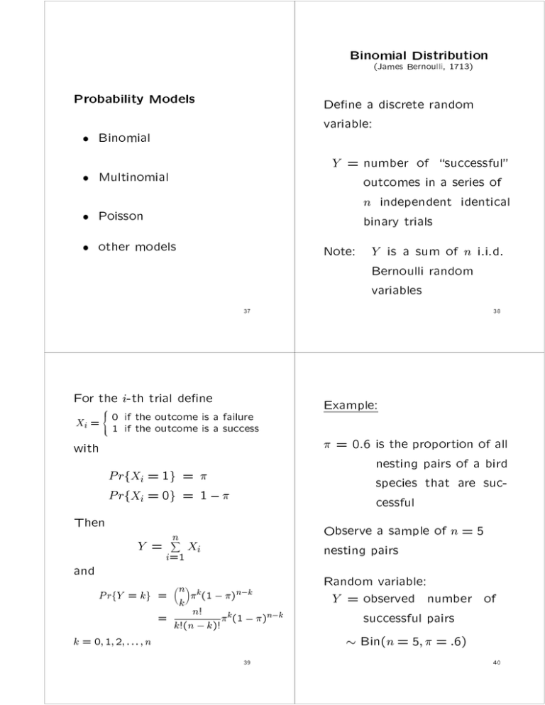
Binomial Distribution
(James Bernoulli, 1713)
Probability Models
Dene a discrete random
variable:
Binomial
Y = number of \successful"
outcomes in a series of
n independent identical
binary trials
Multinomial
Poisson
other models
Note: Y is a sum of n i.i.d.
Bernoulli random
variables
37
For the i-th trial dene
8
<
outcome is a failure
Xi = 01 ifif the
the outcome is a success
38
Example:
:
with
P rfXi = 1g = P rfXi = 0g = 1 Then
Y=
and
n
X
i=1
Observe a sample of n = 5
nesting pairs
Xi
n k
P rfY = kg =
(1 )n k
k
n!
=
k (1 )n k
k!(n k)!
k = 0; 1; 2; : : : ; n
= 0.6 is the proportion of all
nesting pairs of a bird
species that are successful
39
Random variable:
Y = observed number of
successful pairs
Bin(n = 5; = :6)
40
What is the probability of
observing Y = 2 successful
pairs?
5
P r(Y = 2) =
(:6)2(:4)3
2
= (10)(:6)2(:4)3
!
= :2304
Note that
5
5!
=
[2!][(5 2)!]
2
(5)(4)(3)(2)(1)
=
[(2)(1)][(3)(2)(1)]
= 10
!
S
S
S
S
F
F
F
F
F
F
S
F
F
F
S
S
S
F
F
F
F
S
F
F
S
F
F
S
S
F
%
F
F
S
F
F
S
F
S
F
S
F
F
F
S
F
F
S
F
S
S
(.6)(.6)(.4)(.4)(.4)
(.6)(.4)(.6)(.4)(.4)
(.6)(.4)(.4)(.6)(.4)
(.6)(.4)(.4)(.4)(.6)
(.4)(.6)(.6)(.4)(.4)
(.4)(.6)(.4)(.6)(.4)
(.4)(.6)(.4)(.4)(.6)
(.4)(.4)(.6)(.6)(.4)
(.4)(.4)(.6)(.4)(.6)
(.4)(.4)(.4)(.6)(.6)
%
10 ways to
get 2 successes
in n = 5 trials
the probability of
each outcome is
(:6)2(:4)3
41
42
Bin(n = 5; = :6) distribution
5
0
5
1
5
2
5
3
5
4
5
5
P r fY = 1g =
P r fY = 2g =
P r fY = 3g =
P r fY = 4g =
P r fY = 5g =
(:6)0(:4)5 = :01024
P r fY = 0g =
(:6)1(:4)4 = :0768
Mean (or expectation)
E (Y ) = (0)P rfY = 0g + (1)P rfY = 1g
+(2)P rfY = 2g + (3)P rfY = 3g
+(4)P rfY = 4g + (5)P rfY = 5g
(:6)2(:4)3 = :2304
= 3
(:6)3(:4)2 = :3456
(:6)4(:4)1 = :2592
(:6)5(:4)0 = :07776
In general
n
E (Y ) =
k k(1 )n k
k=0 k
= n
n
!
X
Note that 0! is dened as one,
and
5!
5
5!
=
=
=1
0
0!5! (1)(5!)
!
43
%
Sample size
-
population success rate
44
Variance:
V (Y ) =
Moment Generating Function:
n
X
k=0
n
X
(k n)2 P rfY = kg
(k n)2 n k (1 )n k
k
k=0
= n (1 )
=
When Y Bin(n = 5; = :6)
we have
n
X
k=0
etk
n k
(1 )n k
k
= (1 + et)n
g(t)
The r-th moment about zero is
@ r g(t)
E (Y r ) =
@tr
evaluated at t = 0. The r-th central
moment is
V (Y ) = (5)(:6)(:4) = 1:2
The standard deviation is
r
r
E (etY ) =
= V (Y ) = n (1 )
= 1:0954
E (Y
=
r
E (Y ))r
( 1)j r [E (Y )]j E (Y r j )
j
j =0
X
45
46
Third central moment:
E (Y
n)3 =
=
n
X
k=0
n
X
k=0
Skewness:
(k n)3 P rfY = kg
q
(k n)3 n k (1 )n
k
k
1 =
=
= n (1 )(1 2)
Fourth central moment:
E (Y
n)4 =
=
n
X
Kurtosis:
(k n)4 P rfY = kg
k=0
n
X
(k n)4 n k (1 )n
k=0
k
= 3(n (1 ))2
k
+n (1 )(1 6(1 ))
47
2 =
E (Y n)3
[V (Y )]3=2
(1 2)
n (1 )
q
E (Y n)4
[V (Y )]2
= 3 + (1 6(1 ))
n (1 )
48
Inference for Suppose Y is the number of successful
outcomes for a series of n independent
and identical binary trials (simple
random sampling with replacement)
where is the probability of
obtaining a successful outcome on any
single trial (selection).
Y
Bin(n; )
Dene the sample proportion
Y
p=
n
Properties of p = Y=n
maximum likelihood estimator
for E (p) = V (p) = (1n )
p(1 ) N (0; 1), for large n
r
n
r
N (0; 1), for large n
p)
p p(1
n
Note: n is \large" if
n 5 and n(1 ) 5.
49
50
Binomial(10, 0.25) Distribution
0.0
0.0
0.05
0.1
0.10
0.2
0.15
0.20
0.3
0.25
0.4
0.30
Binomial(10, 0.10) Distribution
-2
0
2
4
6
8
10
51
-2
0
2
4
6
8
10
52
Binomial(10, 0.95) Distribution
0.0
0.0
0.1
0.05
0.2
0.10
0.3
0.15
0.4
0.20
0.5
0.6
0.25
Binomial(10, 0.50) Distribution
0
2
4
6
8
10
0
2
4
6
8
10
53
12
54
Binomial(25, 0.10) Distribution
0.0
0.0
0.05
0.1
0.10
0.2
0.15
0.3
0.20
0.4
0.25
Binomial(10, 0.10) Distribution
-2
0
2
4
6
8
10
55
0
5
10
15
20
25
56
Binomial(100, 0.10) Distribution
0.0
0.0
0.02
0.05
0.04
0.06
0.10
0.08
0.10
0.15
0.12
Binomial(50, 0.10) Distribution
0
10
20
30
40
50
0
20
40
60
80
57
Tests of hypotheses:
Example: Is the sex ratio 1:1
for early run Chinook Salmon
caught by hook and line?
count percent
females 172 59.11
males 119 40.89
291
100
58
Test against a two-sided
alternative
null hypothesis H0 : = 0
alternative
HA : 6= 0
Reject H0 if
jZ j = jp (1 0j ) > Z=2
s
Here the estimated proportion of
females is
172
= 0:5911
p=
291
59
0
n
0
is the signicance level (or
type I error level).
60
Example:
Z=
H0 : sex ratio is 1:1
(or = 0 = 0:5)
p 0
0(1 0)
n
=
0:5911 :5
s
(:5)(:5)
291
= 3:107
where is the proportion of
females among all early run
Chinook salmon that could be
caught by hook and line.
p=
s
Since
Z:025 = 1:96
and
Z = 3:107 > 1:96
the null hypothesis is rejected at
the = :05 level of signicance.
172
= 0:5911
291
p-value = .00095 + .00095
= .0019
62
61
/* Program to analyze the 1999 Chinook
salmon data. This program is stored
in the file
chinook1.sas
----------------------- gear=1 run=1 ----------------------The FREQ Procedure
sex
*/
data set1;
infile 'c:\courses\alaska\sas\hdata.dat';
input (year month day biweek run gear
age sex length)
(4. 2. 2. 1. 1. 1. 2. $1. 4.);
rage=int(age/10);
oage=age-(10*rage);
run;
proc sort data=set1; by gear run;
run;
F
M
Frequency
172
119
Percent
Cumulative
Frequency
59.11
40.89
172
291
Cumulative
Percent
59.11
100.00
Binomial Proportion for sex = F
Proportion
ASE
95% Lower Conf Limit
95% Upper Conf Limit
0.5911
0.0288
0.5346
0.6476
Exact Conf Limits
95% Lower Conf Limit
95% Upper Conf Limit
0.5322
0.6481
Test of H0: Proportion = 0.5
ASE under H0
Z
One-sided Pr > Z
Two-sided Pr > |Z|
proc freq data=set1; by gear run;
table sex / binomial (p=.5);
run;
sample size =
63
0.0293
3.1069
0.0009
0.0019
291
64
----------------------- gear=1 run=2 -----------------------
----------------------- gear=2 run=1 -----------------------
The FREQ Procedure
The FREQ Procedure
sex
F
M
Frequency
199
162
Percent
Cumulative
Frequency
55.12
44.88
199
361
Cumulative
Percent
55.12
100.00
sex
Frequency
F
M
165
202
Percent
Cumulative
Frequency
44.96
55.04
165
367
44.96
100.00
Binomial Proportion for sex = F
Binomial Proportion for sex = F
Proportion
ASE
95% Lower Conf Limit
95% Upper Conf Limit
0.5512
0.0262
0.4999
0.6026
Proportion
ASE
95% Lower Conf Limit
95% Upper Conf Limit
0.4496
0.0260
0.3987
0.5005
Exact Conf Limits
95% Lower Conf Limit
95% Upper Conf Limit
0.4983
0.6033
Exact Conf Limits
95% Lower Conf Limit
95% Upper Conf Limit
0.3979
0.5021
Test of H0: Proportion = 0.5
ASE under H0
Z
One-sided Pr > Z
Two-sided Pr > |Z|
Test of H0: Proportion = 0.5
0.0263
1.9474
0.0257
0.0515
ASE under H0
Z
One-sided Pr < Z
Two-sided Pr > |Z|
Sample Size = 361
0.0261
-1.9314
0.0267
0.0534
Sample Size = 367
65
----------------------- gear=2 run=2 ----------------------The FREQ Procedure
sex
F
M
Cumulative
Percent
Frequency
168
268
Percent
Cumulative
Frequency
38.53
61.47
168
436
Cumulative
Percent
An approximate (1-) 100%
condence interval for includes
all values of 0 that satisfy
38.53
100.00
Binomial Proportion for sex = F
r
Proportion
ASE
95% Lower Conf Limit
95% Upper Conf Limit
0.3853
0.0233
0.3396
0.4310
Exact Conf Limits
95% Lower Conf Limit
95% Upper Conf Limit
0.3394
0.4328
Test of H0: Proportion = 0.5
ASE under H0
Z
One-sided Pr < Z
Two-sided Pr > |Z|
66
0.0239
-4.7891
<.0001
<.0001
Sample Size = 436
67
jp 0j < Z
=2
1
n p(1
p)
The upper and lower limits are
pU = p + Z=2
pL = p Z=2
v
u
u
u
t
v
u
u
u
t
p(1 p)
n
p(1 p)
n
68
Example:
(pL; pU ) is not an exact 95%
condence interval because
the binomial distribution is
discrete
bounded
skewed
95% condence interval for proportion of females among early
run salmon that could be caught
with hook and line
=2
Z=2
n
p
a large sample normal
approximation is used
=
=
=
=
=
1 0:95 = :05
:025
1:96
291
172
0:5911 =
291
70
69
v
u
u
t
pU = :5911 + (1:96)
= :6476
v
u
u
t
pL = :5911 (1:96)
= :5346
\Exact" condence intervals:
(:5911)(:4089)
291
(:5911)(:4089)
291
An approximate 95% condence
interval is
(.535, .648)
%
round nal answer to 13 (Std. error for p)
The lower limit is the value of for which
= P r(Y
2
n
y)
n j
(1 )n j
j
j =y
y 1
1
=
t (1 t)n y dt
0
(y; n y + 1)
=
X
Z
I (y; n y + 1)
Note: Use integration by parts with
(a) (b) and (a) = (a 1)!
(a; b) =
(a + b)
s
= 1 (p)(1 p)
3
n
1
= (:0293) = :0097
3
71
72
The upper limit is the value of for which
Note that F = F(v2;v1)=2
satises
v1 v2
= I v1
;
v1+v2 F 2 2
2
0
1
@
A
= P r(Y
2
n j
(1 )n j
j
j =0
n
n j
= 1
(1 )n j
j
j =y+1
=
%
pL =
y
y)
X
X
v1
v1 + v2F(v2;v1);=2
or
where
n
n j
1 =
(1 )n j
2
j
j =y+1
y 1
1
=
t (1 t)n y dt
( y + 1; n y ) 0
X
v1 = 2Y
v2 = 2(n Y + 1)
Z
I (y + 1; n y)
73
74
Since
Note that F = F(v4;v3);1
satises
1 = I v3
2
v4+v3 F
%
pU =
where
=2
v3 v4
;
2 2
1
F(v4;v3);1 =2 =
F
(v3;v4)=2
we have
!
pU =
v3
v4 + v3F(v4;v3);1 =2
v3 F(v3;v4);=2
v4 + v3 F(v3;v4);=2
where
v3 = 2(Y + 1)
v4 = 2(n Y )
v3 = 2(Y + 1)
v4 = 2(n Y )
D. Collette, (1991) Modelling Binary Data, page 25.
Johnson & Kotz (1969), Discrete Distributions, page
59.
75
76
Example:
Observe Y = 1 success
in n = 10 trials
Then
y
p = = 0:10
n
Exact 95% condence interval:
v1 = 2Y = 2
v2 = 2(n Y + 1) = 20
F(20;2):025 = 39:45
Construct a 95% condence
interval for v3 = 2(Y + 1) = 4
Large sample normal approximation
p
1:96 p(1 p)=n
=) 0:10 :186
v4 = 2(n Y ) = 18
q
F(4;18):025 = 3:61
use (0, 0.286)??
78
77
/* This is a SAS/IML program to compute
confidence intervals for a binomial
sucess rate. The program is stored
in the file
The condence limits are
binci.sas
2
pL =
= 0:0025
2 + (20)(39:45)
and
(4)(3:61)
pU =
= 0:445
18 + (4)(3:61)
79
*/
proc iml;
start binci;
x = 1;
n = 10;
a = .95;
* Enter number of successes;
* Enter total number of trials;
* Enter confidence level;
a2=1-((1-a)/2);
v1=x;
v2=n-x+1;
v3=v1+1;
v4=v2-1;
invb1=1;
if(v1 > 0) then invb1 = betainv(a2,v2,v1);
80
invb2=1;
if(v4 > 0) then invb2 = betainv(a2,v3,v4);
pl= 1-invb1;
pu = invb2;
print 'Exact confidence intervals';
print pl pu;
z = probit(a2);
p = v1/n;
pl = p - z*sqrt(p*(1-p)/n);
pu = p + z*sqrt(p*(1-p)/n);
print 'Confidence intervals based on the',
'large sample normal approximation';
print pl pu;
finish;
Exact confidence intervals
PL
PU
0.0025286
0.4450161
Confidence intervals based on the
large sample normal approximation
PL
PU
-0.085939
0.2859385
run binci;
81
#
#
This code is stored in the file
binci.ssc
#
#
#
#
#
#
#
#
#
#
#
#
#
#
This code creates confidence
intervals for a binomial
proportion using
x
n
a
p
#
#
Large sample normal theory
Confidence interval based on
large sample normal theory. This
a2 <- 1-((1-a)/2)
plower <- p - qnorm(a2)*sqrt(p*(1-p)/n)
pupper <- p + qnorm(a2)*sqrt(p*(1-p)/n)
An exact interval
Another approximation
# Round to 5 decimal places and print
# results
x = observed number of successes
n = number of trials
a = level of confidence (e.g. 0.95)
<<<<-
82
round(plower,5)
round(pupper,5)
c(1)
c(10)
c(.95)
x/n
83
84
#
#
#
#
Use quantiles from the F-distribution
to construct an exact confidence interval
The function qf( , , ) computes
quantiles of the F-distribution
a2 <- 1-((1-a)/2)
if (x > 0) f1 <- qf(a2,2*(n-x+1),2*x)
else f1 <- c(1)
plower <- x/(x + (n-x+1)*f1)
if (n > x) f2 <- qf(a2,2*(x+1),2*(n-x))
else f2 <- c(1)
pupper <- (x+1)*f2/((n-x)+(x+1)*f2)
#
#
#
#
#
#
#
#
The prop.test function creates
a confidence using a method
proposed by Fleiss, 2nd ed.
pages 14-15. It also can test
a null hypothesis that the
success rate is a specific value
using the option p=...
prop.test(x,n,conf.level=a,p=.45)
#
#
Print results
To compute and display just
the confidence interval use
prop.test(x,n)$conf.int
round(plower,5)
round(pupper,5)
85
#
#
x
n
a
p
#
#
This is the output for the code
stored in the file
binci.spl
<<<<-
86
#
#
#
#
c(1)
c(10)
c(.95)
x/n
Use quantiles from the F-distribution
to construct an exact confidence interval
The function qf( , , ) computes
quantiles of the F-distribution
a2 <- 1-((1-a)/2)
if (x > 0) f1 <- qf(a2,2*(n-x+1),2*x) else f1 <- c(1
[1] 39.44791
plower <- x/(x + (n-x+1)*f1)
if (n > x) f2 <- qf(a2,2*(x+1),2*(n-x)) else f2 <- c
[1] 3.608344
pupper <- (x+1)*f2/((n-x)+(x+1)*f2)
Confidence interval based on
large sample normal theory. This
a2 <- 1-((1-a)/2)
plower <- p + qnorm(a2)*sqrt(p*(1-p)/n)
pupper <- p - qnorm(a2)*sqrt(p*(1-p)/n)
#
# Round to 5 decimal places and print
# results
Print results
round(plower,5)
[1] 0.00253
round(pupper,5)
[1] 0.44502
round(plower,5)
[1] 0.28594
round(pupper,5)
[1] -0.08594
87
88
#
#
#
#
#
#
#
The prop.test function creates
a confidence using a method
proposed by Fleiss, 2nd ed.
pages 14-15. It also can test
a null hypothesis that the
success rate is a specific value
using the option p=...
95 percent confidence interval:
0.005242302 0.458846016
sample estimates:
prop'n in Group 1
0.1
prop.test(x,n,conf.level=a,p=.45)
Warning messages:
Expected counts < 5. Chi-square/normal
approximation may not be appropriate.
in: prop.test(x, n, conf.level = a, p = 0.45)
1-sample proportions test with continuity
correction
data: x out of n, null
X-square = 3.6364, df =
alternative hypothesis:
Group 1 is not equal to
probability 0.45
1, p-value = 0.0565
true P(success) in
0.45
#
#
To compute and display just
the confidence interval use
prop.test(x,n)$conf.int
[1] 0.005242302 0.458846016
attr(, "conf.level"):
[1] 0.95
89
90
Suppose you observe
Y = 0 successes in n trails,
then
p=
Y
=0
n
and a 95% condence interval
based on the large sample
normal approximation yields
p (1:96) p(1 p)=n
r
Results for "exact" 95%
condence intervals depend
on n:
n
5
10
20
50
100
1000
Lower
Limit
0
0
0
0
0
0
Upper
Limit
.5218
.3085
.1684
.07112
.03622
.003682
=) (0; 0)
91
92
Example: Drinking Survey
In a survey of people aged 18 or over
in England and Wales conducted by
Gallup in 1985, each respondent was
asked
\Thinking about the last 7 days,
on how many of those days did
you have at least one alcoholic
drink?"
Binary response:
Drinker: at least one day
Non-drinker: zero days
Construct a 95% condence interval
for
= proportion of \drinkers" in
18 and over population
Sample size: n = 928
Observed number of drinkers:
Y = 570
Sample proportion: p = 570
928 = :614
Approximate 95% condence interval:
p (1:96) p(1n p)
=) (0:5829; 0:6455)
r
"Exact" method: (0.5820, 0.6457)
94
93
Is a normal approximation to
a binomial distribution an
appropriate model to use in
this case?
Example: Iowa Poll (1999)
Simple random sample with
replacement
plus or minus :035
Simple random sample
without replacement
Cluster sampling
Stratication
95
Sample size: n = 801
Maximum margin of error:
96
How many observations are
needed?
Sample Size (n)
p M = .035 M = .01
.001
4
39
.01
32
381
.1
283
3458
.2
502
6147
.3
659
8068
.4
753
9220
.5
784
9604
.6
753
9220
.7
659
8068
.8
502
6147
.9
283
3458
.99
32
381
.999
4
39
Specify a margin of error
M = 0.035
M = 0.010
Compute n:
v
u
u
u
t
M = (1:96)
=)
p(1 p)
n
1:96 2
n=
p(1 p)
M
2
3
4
5
%
This is maximized when p = 0.5
97
How many observations are needed to
test the null hypothesis H0 : = 0?
Specify a signicance level
(or Type I error level)
= probability of rejecting
H0 : = 0 when H0 is true
Typical values
= .10
= .05
= .01
98
Specify an alternative of
practical importance
H0 : = 0
HA : = A
Specify the desired power of the
test to reject H0 : = 0 when
HA : = A is true.
power = probability that
H0 : = 0 is rejected
when HA : = A is
true.
99
100
Typical values are
power = 0.80
power = 0.90
power = 0.95
Sample size needed to test
H0 : = 0 vs. HA : 6= A
(two sided alternative) is
Type II error probability
= 1 - power
= probability that
H0 : = 0 is not
rejected when
HA : = A is true
q
Derivation of sample size formula:
= power
= P r reject H : = = A
0
n
=
Pr
0
8
>
<
>
:
P
q
+ Pr
=
=
=
Pr
8
>
<
>
:
0
(0 (1
(
n
P
0 )
0
0(1 0 )
n
P
q
0
(0 (1
n
(
0 )
> Z=2 = A
=2
>Z
P r P > 0 + Z=2
Pr
8
>
<
>
:
P
q
%
A
A(1 A )
n
this is approximately
standard normal
>
r
= A
Example:
o
9
>
=
)
9
>
=
>
;
0(1 0) = A
n
0 A + Z=2
q
Want an 80% chance of rejecting the
hypothesis of a 1:1 sex ratio among
salmon caught in nets during the early
run, when at least 58% are female or
less than 42% are female. Will use
= .05 as the Type I error level.
>
;
< Z=2 = A
2
102
101
1
q
Z A(1 A) + Z=2 0(1 0)
n=
[0 A]2
q
)
9
0(1 0 ) >
=
n
A(1 A )
n
>
;
%
this must be the
lower percentile
of the standard
normal distribution
103
H0 : = 0 = :50
HA : 6= 0 and a = :58 or .42
and j0 Aj = .08
104
Sample size for tests against one
sided alternatives:
Signicance level: = .05
Z=2 = Z:025 = 1:96
H0 : = 0 vs. H0 : > 0
power = .80 and
= 1 - power = .20
ZB = Z:20 = :842
q
q
q
Z A(1 A) + Z 0(1 0)
n=
[0 A]2
q
:842 (:58)(:42) + 1:96 (:5)(:5)
n =
[:58 :50]2
= 304:3
2
2
-
round up to n = 305
106
105
SAS and S-PLUS code
SAS and JMP:
No built in function for sample
size determination for binomial
proportions
S-PLUS for Windows:
Click on Statistics
Select Power and Sample Size
Select Binomial Proportion
Fill in the boxes
Click the Options tab and click o
Continuity Correction
Click Okay
SAS code:
/* This program computes sample sizes needed to
obtain a test of a hypothesis about a single
proportion with a specified power value.
It also computes the number of observations
needed to obtain a confidence interval with
a specified accuracy. This program is stored
in the file
size1p.sas
*/
proc iml;
start samples;
p0 = .7;
pa = {.6 .5 .4 .3};
/* Enter alternatives */
power = {.8 .9 .95 .99};
alpha = .05;
107
/* Enter the proportion
corrsponding to the
null hypothesis */
/* Power values */
/* Type I error level */
108
za = probit(1-alpha/2);
za1 = probit(1-alpha);
nb = ncol(power);
np = ncol(pa);
size = j(1,np);
size1 = j(1,np);
print,,,,,,, p0 p2 alpha power;
size = int(size) + j(1,np);
print 'Sample sizes (2-sided test):' size;
print ,,,,,, 'Sample sizes for tests of '
'a single proportion';
do i1 = 1 to np; /* Cycle across alternatives */
p2 = pa[1,i1];
do i2 = 1 to nb; /* Cycle across power levels */
zb = probit(power[1,i2]);
size[1,i2] = ((za*sqrt(p0*(1-p0))
+zb*sqrt(p2*(1-p2)))**2)/((p0-p2)**2);
size1[1,i2] = ((za1*sqrt(p0*(1-p0))
+zb*sqrt(p2*(1-p2)))**2)/((p0-p2)**2);
end;
size = int(size1) + j(1,np);
print 'Sample sizes (1-sided test):' size;
end;
/* Compute sample size needed to obtain a
confidence interval with a specified
margin of error
*/
p = {.5 .4 .3 .2 .1 .01}; /* Enter possible
values of the
true proportion */
level = 0.95;
/* Enter confidence level */
me = { 0.035};
/* Enter desired margin of
error */
109
110
Sample sizes for tests of a single proportion
P0
0.7
/* Compute needed sample sizes */
p = t(p);
alpha2 = (1-level)/2;
np = nrow(p);
n = ((probit(1-alpha2)/me)**2)#p#(j(np,1)-p);
n = int(n) + j(np,1);
ALPHA
0.05
POWER
0.8
percent = level*100;
print ,,,,,, 'Sample sizes for ' percent
'percent confidence interval:';
print p n;
P2
0.6
0.9
0.95
0.99
Sample sizes (2-sided test):
SIZE
172
finish;
233
291
416
Sample sizes (1-sided test):
SIZE
run samples;
136
111
191
244
359
112
P0
P2
ALPHA
P0
P2
ALPHA
0.7
0.5
0.05
0.7
0.4
0.05
POWER
0.8
0.9
POWER
0.95
0.99
0.8
Sample sizes (2-sided test):
SIZE
44
60
75
107
49
63
92
0.95
20
26
33
P2
ALPHA
0.7
0.3
0.05
POWER
0.8
0.9
16
22
28
14
0.95
12
114
0.99
18
25
Sample sizes (1-sided test):
SIZE
9
40
Sample sizes for 95 percent confidence interval:
Sample sizes (2-sided test):
SIZE
11
47
Sample sizes (1-sided test):
SIZE
113
P0
0.99
Sample sizes (2-sided test):
SIZE
Sample sizes (1-sided test):
SIZE
35
0.9
15
P
N
0.5
0.4
0.3
0.2
0.1
0.01
784
753
659
502
283
32
21
115
116
S-PLUS code
#
#
#
#
#
#
#
This program computes sample sizes needed to
obtain a test of a hypothesis about a single
proportion with a specified power value.
It also computes the number of observations
needed to obtain a confidence interval with
a specified accuracy. This program is stored
in the file
size1p.ssc
# Specify the null hypothesis
p0 <- c(.7)
za <- qnorm(1-alpha/2)
za1 <- qnorm(1-alpha)
nb <- length(power)
np <- length(pa)
cat("Sample sizes for tests of a single proportion")
# Cycle across the list of alternatives
# and obtain a sample size for each of
# the requested power values
for(i1 in 1:np){
p2 <- pa[i1]
zb <- qnorm(power)
size <- ((za*sqrt(p0*(1-p0))
+zb*sqrt(p2*(1-p2)))^2)/((p0-p2)^2)
size1 <- ((za1*sqrt(p0*(1-p0))
+zb*sqrt(p2*(1-p2)))^2)/((p0-p2)^2)
# Enter a vector of alternatives
pa <- c(.6, .5, .4, .3)
# Enter power values
power <- c(.8, .9, .95, .99)
# Ener the type I error level
alpha <- .05
117
# Increase sample size to next largest integer
# and print results
size <- ceiling(size)
cat("\n \n \n p0=",p0,"pA=", p2, "alpha=",
alpha,"power=", power)
cat("\n Sample sizes (2-sided test): " , size)
size1 <- ceiling(size1)
cat("\n \n p0=",p0,"pA=", p2, "alpha=",
alpha,"power=", power)
cat("\n Sample sizes (1-sided test): " , size1)
}
# Compute sample size needed to obtain a
# confidence interval with a specified
# margin of error
# Enter possible values of the true proportion
p <- c(.5, .4, .3, .2, .1, .01)
118
# Enter desired margin of error
me <- c(0.035)
# Compute needed sample sizes
alpha2 <- (1.0-level)/2
np <- length(p)
one <- rep(1,np)
n <-((qnorm(one-alpha2)/me)^2)*p*(one-p)
n <- ceiling(n)
sizes<-t(rbind(p,n))
percent <- level*100
cat("\n \n \n Sample sizes for", percent,
"percent confidence intervals \n",
"with margin of error ", me, "\n")
sizes
# Enter the confidence level
level <- c(0.95)
119
120
# This is the output from the S-PLUS code
# in the file size1p.ssc.
Sample sizes for tests of a single proportion
p0= 0.7 pA= 0.6 alpha= 0.05
power= 0.8 0.9 0.95 0.99
Sample sizes (2-sided test): 172 233 291 416
p0= 0.7 pA= 0.6 alpha= 0.05
power= 0.8 0.9 0.95 0.99
Sample sizes (1-sided test): 136 191 244 359
p0= 0.7 pA= 0.5 alpha= 0.05
power= 0.8 0.9 0.95 0.99
Sample sizes (2-sided test): 44 60 75 107
p0= 0.7 pA= 0.5 alpha= 0.05
power= 0.8 0.9 0.95 0.99
Sample sizes (1-sided test): 35 49 63 92
121
Sample sizes for 95 percent confidence intervals
with margin of error 0.035
[1,]
[2,]
[3,]
[4,]
[5,]
[6,]
p
0.50
0.40
0.30
0.20
0.10
0.01
n
784
753
659
502
283
32
123
p0= 0.7 pA= 0.4 alpha= 0.05
power= 0.8 0.9 0.95 0.99
Sample sizes (2-sided test): 20 26 33 47
p0= 0.7 pA= 0.4 alpha= 0.05
power= 0.8 0.9 0.95 0.99
Sample sizes (1-sided test): 16 22 28 40
p0= 0.7 pA= 0.3 alpha= 0.05
power= 0.8 0.9 0.95 0.99
Sample sizes (2-sided test): 11 14 18 25
p0= 0.7 pA= 0.3 alpha= 0.05
power= 0.8 0.9 0.95 0.99
Sample sizes (1-sided test): 9 12 15 21
122