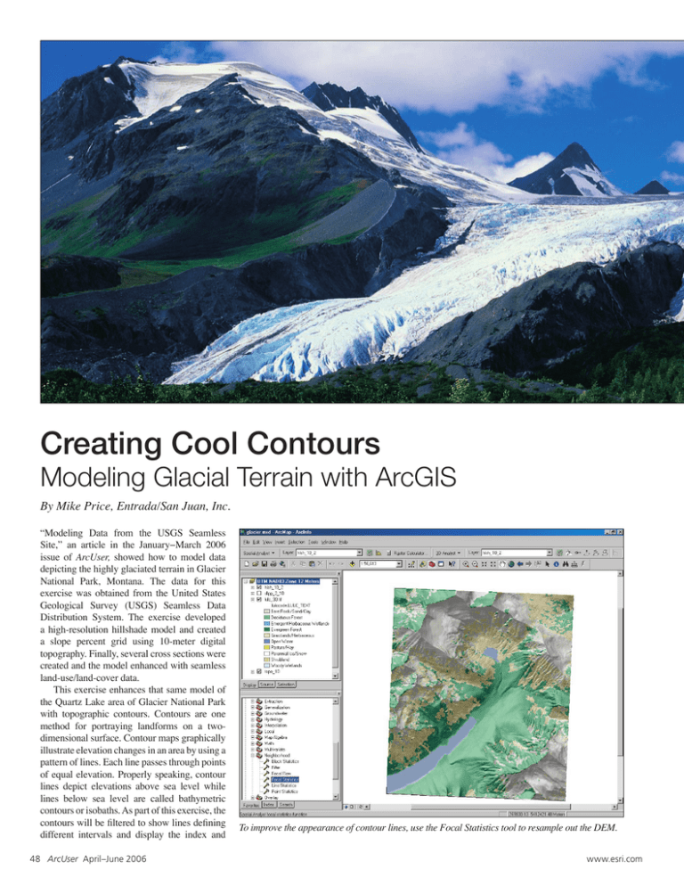
Creating Cool Contours
Modeling Glacial Terrain with ArcGIS
By Mike Price, Entrada/San Juan, Inc.
“Modeling Data from the USGS Seamless
Site,” an article in the January−March 2006
issue of ArcUser, showed how to model data
depicting the highly glaciated terrain in Glacier
National Park, Montana. The data for this
exercise was obtained from the United States
Geological Survey (USGS) Seamless Data
Distribution System. The exercise developed
a high-resolution hillshade model and created
a slope percent grid using 10-meter digital
topography. Finally, several cross sections were
created and the model enhanced with seamless
land-use/land-cover data.
This exercise enhances that same model of
the Quartz Lake area of Glacier National Park
with topographic contours. Contours are one
method for portraying landforms on a twodimensional surface. Contour maps graphically
illustrate elevation changes in an area by using a
pattern of lines. Each line passes through points
of equal elevation. Properly speaking, contour
lines depict elevations above sea level while
lines below sea level are called bathymetric
contours or isobaths. As part of this exercise, the
contours will be filtered to show lines defining
different intervals and display the index and
To improve the appearance of contour lines, use the Focal Statistics tool to resample out the DEM.
48 ArcUser April–June 2006
www.esri.com
Hands On
What You Will Need
• ArcGIS 9x (ArcView, ArcEditor, or ArcInfo)
• ArcGIS 9 Spatial Analyst extension
• Sample dataset from ArcUser Online
intermediate contours without having to create
data subsets.
Setting Up the Project
Download the sample dataset from ArcUser
Online
(www.esri.com/arcuser).
When
unzipped, it should generate a directory
structure. The root folder contains a completed
version of the Quartz Lake model for Glacier
National Park called Glacier01.mxd and the
additional files that will be used.
Smoothing a DEM
with a Focal Neighborhood
Building a topography contour set from raw
digital elevation model (DEM) data creates a
contour set that can show the minor variations
and irregularities in the data caused by DEM
seaming and registration artifacts. In flat areas,
contour lines can be very linear and angular.
To create a smooth contour set for topography
and other grids, it is helpful and relevant to
slightly smooth the data before contouring.
The smoothed grid should be named and
documented with information describing the
smoothing process used. This grid should not
be used for any analysis that requires raw DEM
data.
1. Open
Glacier01.mxd
and
display
ArcToolbox. Make the ArcGIS Spatial Analyst
extension active.
2. To smooth the topo_10 grid, access
ArcToolbox and select Spatial Analyst toolbox
> Neighborhood tools > Focal Statistics. The
In the the Focal Statistics wizard, specify the shape and radius of the neighborhood.
Focal Statistics tool will resample out the DEM
and apply a search distance defined by cells or
model distance.
3. In the wizard, specify topo_10 as the Input
raster and name the Output raster \Glacier\
GRDFiles\LatLon\topo_10s2.
4. Select Circle from the drop-down next to
Neighborhood and set the smoothing Radius to
2. Leave all other default settings.
5. Specify MEAN as the Statistics type. Click
www.esri.com
OK to create the smoothed grid and watch it
load. Notice that it is a 10-meter floating-point
terrain set with the same extent as topo_10.
Contouring DEM Data
Contour lines can be created from this smoothed
grid.
1. Open the Spatial Analyst’s Surface toolset
and select Contours.
Continued on page 50
ArcUser April–June 2006 49
Creating Cool Contours
Modeling Glacial Terrain with ArcGIS
Continued from page 49
2. Select topo_10s2 as the Input raster and
specify \Glacier\SHPFiles\LatLon\topocon05s2
as the Output polyline features. Make sure to
change the output to the SHPFiles folder.
3. Set the Contour Interval to five meters and
leave default values for other options. Click OK
to create the contours.
When the contours have drawn, zoom in
and inspect them. Notice that these lines are
quite dense, especially when the entire model
is viewed. Open the attribute table and verify
that approximately 1,841 contour lines were
created. These contours range in elevation from
1,350 to 4,000 meters.
Joining a Contour Filter Lookup Table
The contour set uses a five-meter elevation
interval. For large-scale mapping, this might
be an appropriate resolution, but for maps with
this project’s extent, this is probably too dense.
It would be nice to be able to quickly filter these
contours to show only lines defining intervals of
10, 20, 50, or other similar interval. The dataset
for this tutorial supplies a lookup table that
quickly filters contours without creating data
subsets. This table applies binary codes (0 and
1) to identify and filter out unneeded lines. In
addition, with the same lookup table, index and
intermediate contours can easily be displayed
from within the same set.
Navigate to \Glacier\Utility\ and add Cont_
Sel.dbf to the map. Click on the Sources tab in
the Table of Contents and right-click on Cont_
Sel.dbf. This table contains records for more
than 3,000 continuous five-unit elevation slices,
ranging from -350 to 15,000. It is designed to
work with any continental United States data
that is posted in feet. For models in Z meters,
this set will work anywhere in the world.
Cont_Sel.dbf contains an elevation field
(ELEV_BASE) followed by a series of selection
fields populated with 0 or 1. If an elevation
value is evenly divisible by the contour interval
named in the field (e.g., 410 is evenly divisible
by 5, and 10, but not by 20), the appropriate
field contains a value of 1; if it is not evenly
divisible, it contains a 0. Contour filters are
set at values of 5, 10, 20, 25, 40, 50, 100, 200,
250, and 500 so they can be used to filter raw
data contoured with one- or two-unit intervals.
Apply this table by joining it to the new contour
set. Use a selected join field to filter the data.
1. In the Table of Contents, right-click on
topocon05s2 and choose Joins and Relates >
Join.
2. In the Join Data window, specify
CONTOUR as the field that the join will be
based on. Choose cont_sel as the table to join,
and set ELEV_BASE as the field in the table to
base the join on.
3. Click OK to finish. Inspect the join and
verify that the fields are properly assigned.
Filtering Extra Contours
Now create 20-foot interval contours for the
Glacier National Park.
1. Right-click topocon05s2 and open
Properties.
2. Select the Definition Query tab. Click on the
Query Builder button.
3. Use Query Builder to create the expression
“Cont_Sel.ELEV_020” = 1 in the calculation
window. Click OK twice to effect the change.
4. Reopen the contour attribute table and verify
that there are now 493 entities in the filtered
20-meter set. Visually inspect the model to
confirm that the interval is appropriate for this
scale.
The sample dataset contains a lookup table that quickly filters contours without creating data
subsets.
The lookup table applies binary codes (0 and 1) to identify and filter out unneeded lines.
50 ArcUser April–June 2006
www.esri.com
Hands On
In the Join Data window, specify CONTOUR
as the field that the join will be based on.
Choose cont_sel as the table to join, and set
ELEV_BASE as the field in the table to base
the join on.
Coding Index
and Intermediate Contours
Contour maps often apply a system of index
and intermediate contour lines to emphasize
regional trends while still providing detail.
It is standard practice to highlight one index
contour for every fifth contour interval. Since
the contour lines have been filtered with a
20-unit interval, lines should be displayed every
100 units. The same tabular join that was used
to filter the original contour set will also allow
mapping of multiple contour line types.
1. Double-click on topocon05s2 to reopen
the Properties dialog box and click on the
Symbology tab.
2. Select Categories, then Unique Values
legend and set cont.sel.ELEV_100 as the Value
Field.
3. Click Add All Values and verify that 0 and 1
will be the values mapped.
4. Right-click on 0 and choose Reverse Sorting
from the context menu to make 1 first in the
legend.
5. Click on the Label column and label 1 as
Index Contours. Use the same procedure to
label 0 as Intermediate Contours. Uncheck <all
other values>.
6. Select a dark brown color for both line types.
Set a thickness of 1.2 points for Index Contours
and 0.6 points for Intermediate Contours.
7. Click OK twice to apply the new legend and
inspect the map. And all this was done with just
one contour dataset.
The five-meter elevation interval is too dense for this extent.
Contour maps often apply a system of index and intermediate contour lines. Use the lookup table
to filter the contours at 20-unit intervals and set index lines every 100 units.
For Bonus Points
To make this exercise more robust, go back
and refilter the contour set at the 40- and 50meter intervals and redisplay index contours at
200 and 250 units. Use this technique with other
types of grid data that can be contoured such as
thickness, precipitation, population density, and
geophysical data.
www.esri.com
Summary
ArcGIS, with the Spatial Analyst extension,
provides powerful analytical, cartographic, and
visualization tools to model, map, and display
complex geomorphic terrains. To improve the
appearance of the contours, slightly smoothed
data was employed. Rather than creating new
data, this data was filtered and reused.
ArcUser April–June 2006 51