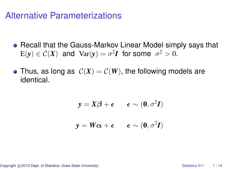
Alternative Parameterizations
advertisement

Alternative Parameterizations
Recall that the Gauss-Markov Linear Model simply says that
E(y) ∈ C(X) and Var(y) = σ 2 I for some σ 2 > 0.
Thus, as long as C(X) = C(W), the following models are
identical.
y = Xβ + ∼ (0, σ 2 I)
y = Wα + ∼ (0, σ 2 I)
c
Copyright 2010
Dept. of Statistics (Iowa State University)
Statistics 511
1 / 14
For example
i = 1, 2, 3
yij
j = 1, 2
Treatment Effects
E(yij ) = µ + τi
1
1
1
1
1
1
1
1
0
0
0
0
X
0
0
1
1
0
0
0
0
0
0
1
1
Cell Means
E(yij ) = µi
µ
τ1
τ2
τ3
β
c
Copyright 2010
Dept. of Statistics (Iowa State University)
1
1
0
0
0
0
0
0
1
1
0
0
W
0
0
0
0
1
1
µ1
µ2
µ3
α
Statistics 511
2 / 14
Both models state that
E(y) ∈
a1
a1
a2
a2
a3
a3
·
·
a1 , a2 , a3 ∈ IR
= C(X) = C(W).
Thus, the two models are identical.
c
Copyright 2010
Dept. of Statistics (Iowa State University)
Statistics 511
3 / 14
In models like the treatment effects model where the design
matrix is not of full column rank, “identifiability constraints”
are often imposed.
The most common constraints are
“set first to zero” τ1 = 0
R default
“set last to zero”
τ3 = 0
SAS effective default
“sum to zero”
τ1 + τ2 + τ3 = 0
c
Copyright 2010
Dept. of Statistics (Iowa State University)
Statistics 511
4 / 14
Such constraints are not necessary.
Placing such constriants on the parameters can be viewed
as equivalent to choosing a particular full column rank
design matrix.
Set first to zero:
1
1
1
1
1
1
0
0
1
1
0
0
0
0
0
0
1
1
c
Copyright 2010
Dept. of Statistics (Iowa State University)
µ
τ2 =
τ
3
µ
µ
µ + τ2
µ + τ2
µ + τ3
µ + τ3
Statistics 511
5 / 14
Set last to zero:
1
1
1
1
1
1
1
1
0
0
0
0
0
0
1
1
0
0
µ
τ
=
1
τ2
Sum to zero: τ1 + τ2 + τ3 = 0 ⇐⇒ τ3
1
1
0
1
0
1
µ
0
1
1
τ1 =
0
1
1
1 −1 −1 τ2
1 −1 −1
c
Copyright 2010
Dept. of Statistics (Iowa State University)
µ + τ1
µ + τ1
µ + τ2
µ + τ2
µ
µ
= −τ1 − τ2
µ + τ1
µ + τ1
µ + τ2
µ + τ2
µ − τ1 − τ2
µ − τ1 − τ2
Statistics 511
6 / 14
Instead of viewing “identifiability constraints” as constraints
on parameters, we can view them as constraints on our
solutions to the normal equations.
For example,
X=
1
1
1
1
1
1
1
1
0
0
0
0
0
0
1
1
0
0
0
0
0
0
1
1
c
Copyright 2010
Dept. of Statistics (Iowa State University)
µ
τ1
β=
τ2
τ3
y=
y11
y12
y21
y22
y31
y33
Statistics 511
7 / 14
Normal Equations X0 Xb = X0 y
?
n· n1 n2 n3
n1 n1 0 0 ?
n2 0 n2 0 ?
?
n3 0 0 n3
Set first to zero
ȳ1·
0
ȳ2· − ȳ1·
ȳ3· − ȳ1·
Set last to zero
ȳ3·
ȳ1· − ȳ3·
ȳ2· − ȳ3·
0
c
Copyright 2010
Dept. of Statistics (Iowa State University)
y··
y1·
=
y2·
y3·
Sum to zero
(ȳ1· + ȳ2· + ȳ3· )/3
ȳ1· − (ȳ1· + ȳ2· + ȳ3· )/3
ȳ2· − (ȳ1· + ȳ2· + ȳ3· )/3
ȳ3· − (ȳ1· + ȳ2· + ȳ3· )/3
Statistics 511
8 / 14
As noted before, such constraints are not necessary; we do
not need to consider constraints when we work with
generalized inverses.
In 611, we study the issue of constraints much more
carefully. We show that constraints of the form Mb = 0
produce a unique solution to the normal equations without
restricting that solution to a proper subset of C(X) if and only
if
C(X0 ) ∩ C(M0 ) = {0} and rank(M) = p − rank(X).
Such constraints have no impact on what linear functions of
β are estimable or on inferences about estimable functions
of β. Thus, the same analysis results are obtained with or
without constraints.
c
Copyright 2010
Dept. of Statistics (Iowa State University)
Statistics 511
9 / 14
In 511, we often start with a non-full-rank design matrix for
ease and symmetry when specifying a model.
For example, it is nice to be able to write
yijk = µ + αi + βj + ijk for i = 1, 2, 3; j = 1, 2, 3, 4; k = 1, . . . , 10
if we want to specify a two-factor additive model.
The design matrix that matches this model specification
does not have full-column rank.
R (and other statistical software) will automatically pick a
full-column-rank design matrix, which is equivalent to placing
certain constraints on the solutions to the normal equations.
c
Copyright 2010
Dept. of Statistics (Iowa State University)
Statistics 511
10 / 14
It does not matter which full-column-rank design matrix (or
corresponding constraint set) is chosen as long as the
column space of the selected design matrix is the same as
the column space of the design matrix for the model as
originally specified.
However, it is important to understand the design matrix
used so that the parameter estimates corresponding to
coefficients in the linear combination of the columns of the
design matrix can be properly interpreted.
c
Copyright 2010
Dept. of Statistics (Iowa State University)
Statistics 511
11 / 14
For example, suppose E(yij ) = µ + τi for i = 1, 2, 3 and
j = 1, . . . , ni
What does the parameter τ2 represent?
Constraints
none
set first to zero
set last to zero
sum to zero
Interpretation of τ2
non-estimable
trt 2 mean − trt 1 mean
trt 2 mean − trt 3 mean
trt 2 mean − average of trt 1, 2, 3 means
c
Copyright 2010
Dept. of Statistics (Iowa State University)
Statistics 511
12 / 14
Recall that all linear functions of E(y) are the only estimable
quantities; i.e., the estimable quantities are given by
{AE(y) : A an n-column matrix of constants}.
Thus, as long as models restrict E(y) to the same column
space, the estimable quantities are identical.
c
Copyright 2010
Dept. of Statistics (Iowa State University)
Statistics 511
13 / 14
Then why, in the treatment effects formulation of the model,
is it that τ2 is estimable under “set first to zero” constraint but
not estimable without constraints?
Under “set first to zero” constraint, τ2 is the estimable
quantity “treatment 2 mean − treatment 1 mean.”
With no constraints, that same quantity is also estimable, but
it is τ2 − τ1 .
c
Copyright 2010
Dept. of Statistics (Iowa State University)
Statistics 511
14 / 14


