Examining Residuals in Simple Linear Regression
Consider the simple linear regression model Yi = β0 + β1 Xi + ei where the error terms e1 , . . . , en are independent normal
random variables with mean 0 and standard deviation σ.
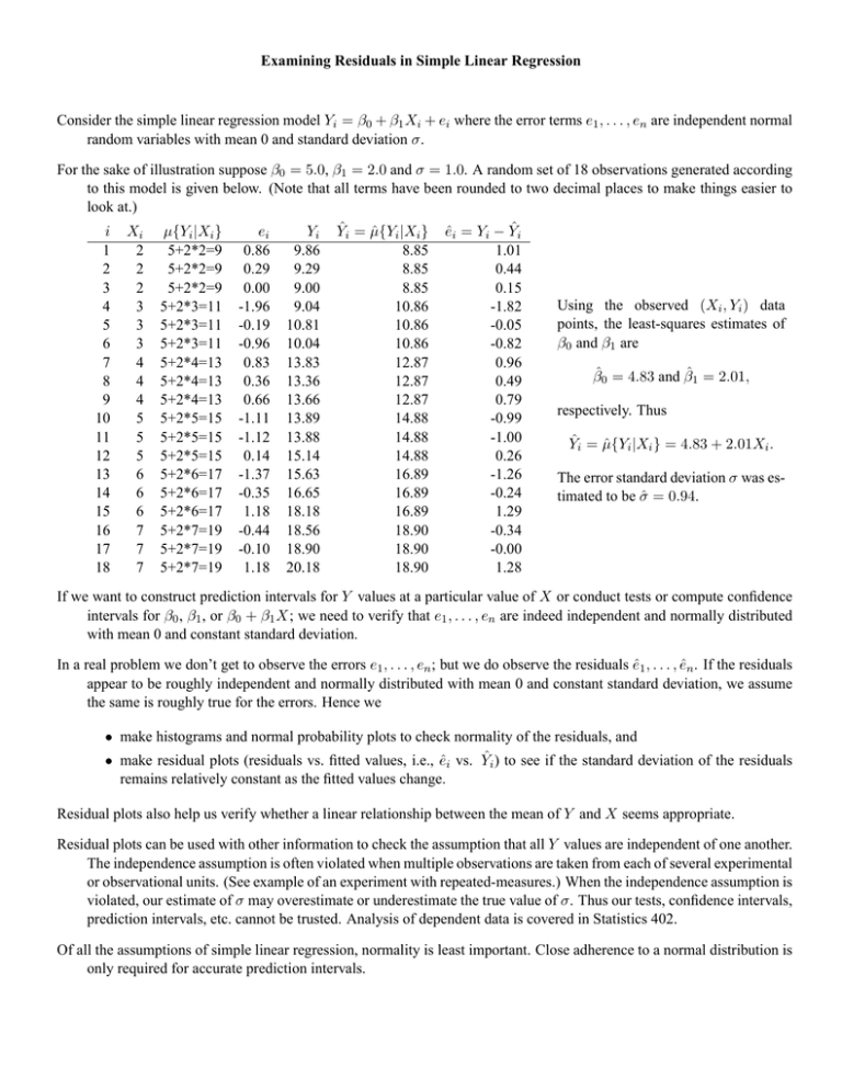
For the sake of illustration suppose β0 = 5.0, β1 = 2.0 and σ = 1.0. A random set of 18 observations generated according
to this model is given below. (Note that all terms have been rounded to two decimal places to make things easier to
look at.)
i
1
2
3
4
5
6
7
8
9
10
11
12
13
14
15
16
17
18
Xi
2
2
2
3
3
3
4
4
4
5
5
5
6
6
6
7
7
7
µ{Yi |Xi }
5+2*2=9
5+2*2=9
5+2*2=9
5+2*3=11
5+2*3=11
5+2*3=11
5+2*4=13
5+2*4=13
5+2*4=13
5+2*5=15
5+2*5=15
5+2*5=15
5+2*6=17
5+2*6=17
5+2*6=17
5+2*7=19
5+2*7=19
5+2*7=19
ei
0.86
0.29
0.00
-1.96
-0.19
-0.96
0.83
0.36
0.66
-1.11
-1.12
0.14
-1.37
-0.35
1.18
-0.44
-0.10
1.18
Yi
9.86
9.29
9.00
9.04
10.81
10.04
13.83
13.36
13.66
13.89
13.88
15.14
15.63
16.65
18.18
18.56
18.90
20.18
Ŷi = µ̂{Yi |Xi }
8.85
8.85
8.85
10.86
10.86
10.86
12.87
12.87
12.87
14.88
14.88
14.88
16.89
16.89
16.89
18.90
18.90
18.90
êi = Yi − Ŷi
1.01
0.44
0.15
-1.82
-0.05
-0.82
0.96
0.49
0.79
-0.99
-1.00
0.26
-1.26
-0.24
1.29
-0.34
-0.00
1.28
Using the observed (Xi , Yi ) data
points, the least-squares estimates of
β0 and β1 are
β̂0 = 4.83 and β̂1 = 2.01,
respectively. Thus
Ŷi = µ̂{Yi |Xi } = 4.83 + 2.01Xi .
The error standard deviation σ was estimated to be σ̂ = 0.94.
If we want to construct prediction intervals for Y values at a particular value of X or conduct tests or compute confidence
intervals for β0 , β1 , or β0 + β1 X; we need to verify that e1 , . . . , en are indeed independent and normally distributed
with mean 0 and constant standard deviation.
In a real problem we don’t get to observe the errors e1 , . . . , en ; but we do observe the residuals ê1 , . . . , ên . If the residuals
appear to be roughly independent and normally distributed with mean 0 and constant standard deviation, we assume
the same is roughly true for the errors. Hence we
• make histograms and normal probability plots to check normality of the residuals, and
• make residual plots (residuals vs. fitted values, i.e., êi vs. Ŷi ) to see if the standard deviation of the residuals
remains relatively constant as the fitted values change.
Residual plots also help us verify whether a linear relationship between the mean of Y and X seems appropriate.
Residual plots can be used with other information to check the assumption that all Y values are independent of one another.
The independence assumption is often violated when multiple observations are taken from each of several experimental
or observational units. (See example of an experiment with repeated-measures.) When the independence assumption is
violated, our estimate of σ may overestimate or underestimate the true value of σ. Thus our tests, confidence intervals,
prediction intervals, etc. cannot be trusted. Analysis of dependent data is covered in Statistics 402.
Of all the assumptions of simple linear regression, normality is least important. Close adherence to a normal distribution is
only required for accurate prediction intervals.