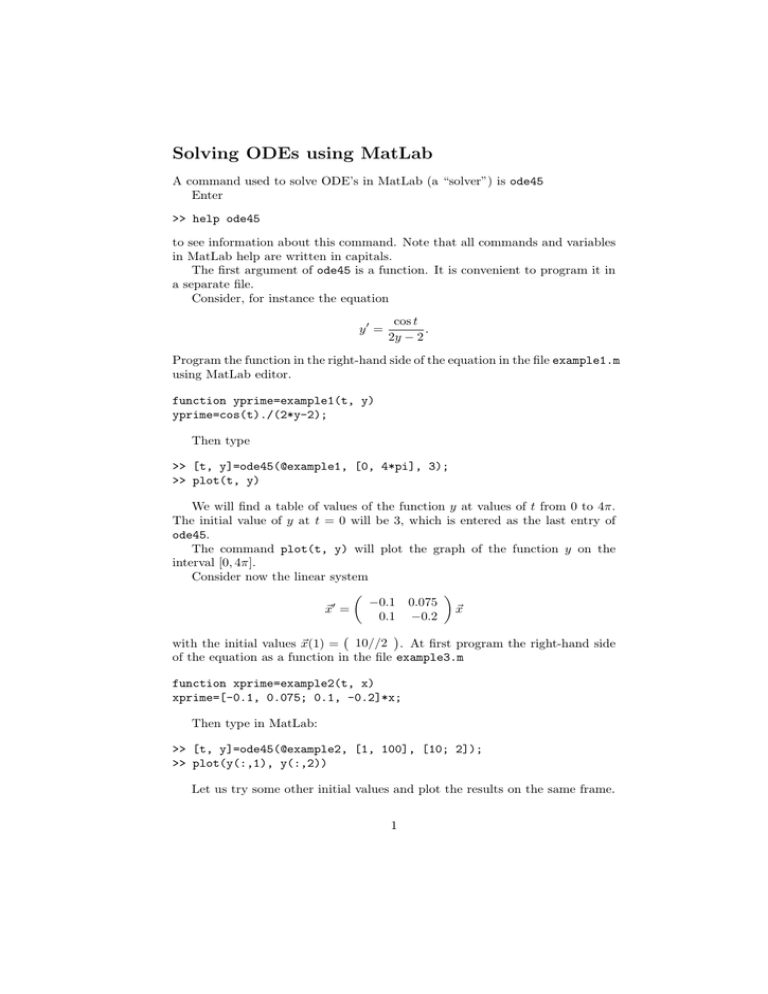
Solving ODEs using MatLab
A command used to solve ODE’s in MatLab (a “solver”) is ode45
Enter
>> help ode45
to see information about this command. Note that all commands and variables
in MatLab help are written in capitals.
The first argument of ode45 is a function. It is convenient to program it in
a separate file.
Consider, for instance the equation
y0 =
cos t
.
2y − 2
Program the function in the right-hand side of the equation in the file example1.m
using MatLab editor.
function yprime=example1(t, y)
yprime=cos(t)./(2*y-2);
Then type
>> [t, y]=ode45(@example1, [0, 4*pi], 3);
>> plot(t, y)
We will find a table of values of the function y at values of t from 0 to 4π.
The initial value of y at t = 0 will be 3, which is entered as the last entry of
ode45.
The command plot(t, y) will plot the graph of the function y on the
interval [0, 4π].
Consider now the linear system
−0.1 0.075
~x0 =
~x
0.1 −0.2
with the initial values ~x(1) = 10//2 . At first program the right-hand side
of the equation as a function in the file example3.m
function xprime=example2(t, x)
xprime=[-0.1, 0.075; 0.1, -0.2]*x;
Then type in MatLab:
>> [t, y]=ode45(@example2, [1, 100], [10; 2]);
>> plot(y(:,1), y(:,2))
Let us try some other initial values and plot the results on the same frame.
1
>> hold
Current plot held
>> [t, y]=ode45(@example2,
>> plot(y(:,1), y(:,2))
>> [t, y]=ode45(@example2,
>> plot(y(:,1), y(:,2))
>> [t, y]=ode45(@example2,
>> plot(y(:,1), y(:,2))
>> [t, y]=ode45(@example2,
>> plot(y(:,1), y(:,2))
>> [t, y]=ode45(@example2,
>> plot(y(:,1), y(:,2))
[1, 100], [10; -2]);
[1, 100], [0; 10]);
[1, 100], [5; 6]);
[1, 100], [-10; 0]);
[1, 100], [-10; -10]);
Consider now the system
~x0 =
>>
>>
>>
>>
>>
>>
−0.5
−1
1
−0.5
~x
hold off
[t, y]=ode45(@example3, [1, 100], [1; 0]);
plot(y(:,1), y(:,2))
hold Current plot held
[t, y]=ode45(@example3, [1, 100], [-2; 0]);
plot(y(:,1), y(:,2))
If we want to solve a second order ODE, we have to pass to the equivalent
first order system. For example, if we want to solve the equation
4t2 y 00 + 8ty + 65y = 0,
we pass to the system
y10
y20
= y2
= −2y2 /t − 65y1 /(4t2 )
where y1 = y and y2 = y 0 . So, we define a function example4
function xprime=example4(t, x)
xprime=[0; 0];
xprime(1)=x(2);
xprime(2)=-2*x(2)/t-65*x(1)/(4*t^2);
>>
>>
>>
>>
>>
>>
>>
hold off
[t, y]=ode45(@example4, [1, 3*pi], [2; 3]);
plot(t, y(:,1))
[t, y]=ode45(@example4, [1, 6*pi], [2; 3]);
plot(t, y(:,1))
[t, y]=ode45(@example4, [1, 20*pi], [2; 3]);
plot(t, y(:,1))
2
Below are some other examples. Download the m-files and see what functions
they describe.
>> [t, y]=ode45(@example5,
>> plot(t, y(:,1))
>> [t, y]=ode45(@example6,
>> plot(t, y(:,1))
>> hold
Current plot held
>> [t, y]=ode45(@example6,
>> plot(t, y(:,1))
>> [t, y]=ode45(@example6,
>> plot(t, y(:,1))
>> [t, y]=ode45(@example6,
>> plot(t, y(:,1))
>> hold off
>> [t, y]=ode45(@example7,
>> plot(t, y(:,1))
>> [t, y]=ode45(@example7,
>> plot(t, y(:,1))
>> [t, y]=ode45(@example7,
>> plot(t, y(:,1))
>> [t, y]=ode45(@example7,
>> plot(t, y(:,1))
[0, 3], [2; 3]);
[0, 2], [1; -4]);
[0, 2], [1; -2]);
[0, 2], [1; 0]);
[0, 2], [1; 2]);
[-1, 2], [1; 1]);
[-1, 10], [1; 1]);
[-1, 13], [1; 1]);
[-3, 13], [1; 1]);
3