Math 308, Matlab assignment 4
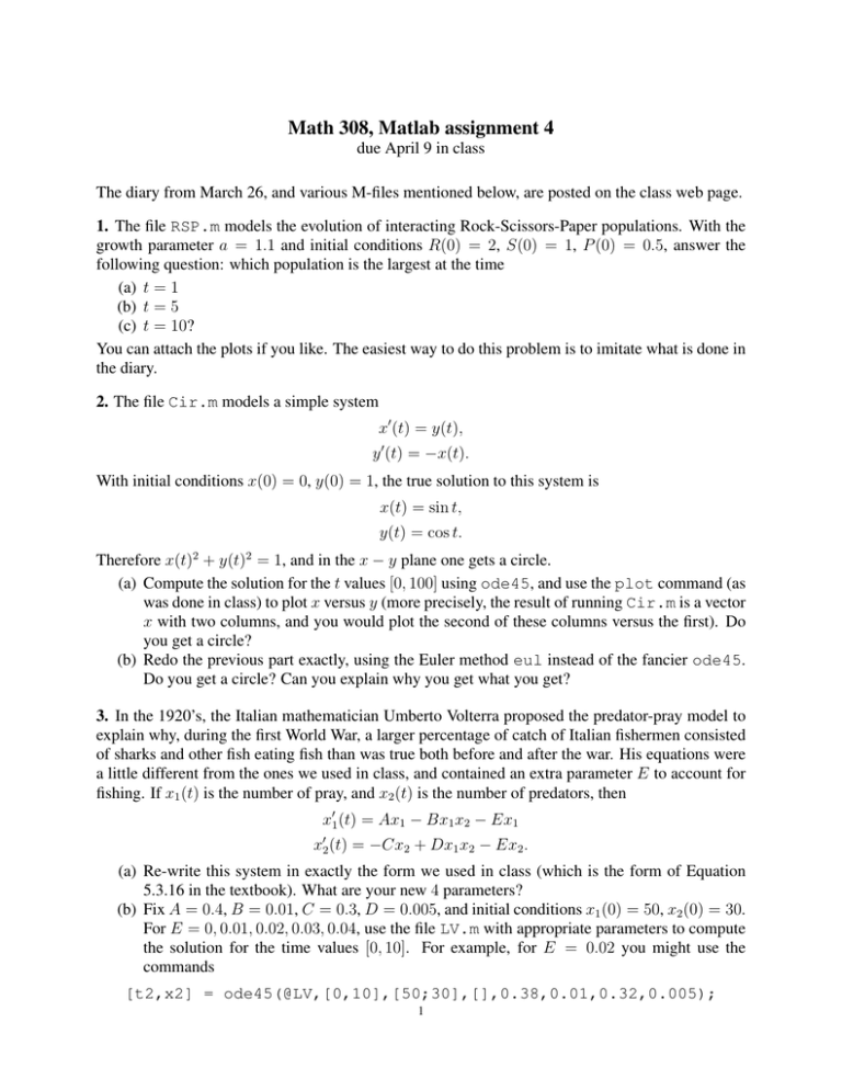
due April 9 in class
The diary from March 26, and various M-files mentioned below, are posted on the class web page.
1. The file RSP.m models the evolution of interacting Rock-Scissors-Paper populations. With the
growth parameter a = 1.1 and initial conditions R(0) = 2, S(0) = 1, P (0) = 0.5, answer the
following question: which population is the largest at the time
(a) t = 1
(b) t = 5
(c) t = 10?
You can attach the plots if you like. The easiest way to do this problem is to imitate what is done in
the diary.
2. The file Cir.m models a simple system
x0 (t) = y(t),
y 0 (t) = −x(t).
With initial conditions x(0) = 0, y(0) = 1, the true solution to this system is
x(t) = sin t,
y(t) = cos t.
Therefore x(t)2 + y(t)2 = 1, and in the x − y plane one gets a circle.
(a) Compute the solution for the t values [0, 100] using ode45, and use the plot command (as
was done in class) to plot x versus y (more precisely, the result of running Cir.m is a vector
x with two columns, and you would plot the second of these columns versus the first). Do
you get a circle?
(b) Redo the previous part exactly, using the Euler method eul instead of the fancier ode45.
Do you get a circle? Can you explain why you get what you get?
3. In the 1920’s, the Italian mathematician Umberto Volterra proposed the predator-pray model to
explain why, during the first World War, a larger percentage of catch of Italian fishermen consisted
of sharks and other fish eating fish than was true both before and after the war. His equations were
a little different from the ones we used in class, and contained an extra parameter E to account for
fishing. If x1 (t) is the number of pray, and x2 (t) is the number of predators, then
x01 (t) = Ax1 − Bx1 x2 − Ex1
x02 (t) = −Cx2 + Dx1 x2 − Ex2 .
(a) Re-write this system in exactly the form we used in class (which is the form of Equation
5.3.16 in the textbook). What are your new 4 parameters?
(b) Fix A = 0.4, B = 0.01, C = 0.3, D = 0.005, and initial conditions x1 (0) = 50, x2 (0) = 30.
For E = 0, 0.01, 0.02, 0.03, 0.04, use the file LV.m with appropriate parameters to compute
the solution for the time values [0, 10]. For example, for E = 0.02 you might use the
commands
[t2,x2] = ode45(@LV,[0,10],[50;30],[],0.38,0.01,0.32,0.005);
1
For each of the solutions, plot the number of pray versus the number of predators, all on the
same plot, and label them appropriately.
(c) Finally, plot on the same graph the ratio of the predators to the pray for each of your five
solutions. You would use something like
plot(t0,x0(:,1)./x0(:,2),t1,x1(:,1)./x1(:,2),t2,x2(:,1)./x2(:,2),
t3,x3(:,1)./x3(:,2),t4,x4(:,1)./x4(:,2)); shg
(depending on your own notation). During the war, the total amount of fishing (the value of
the parameter E) decreased. Does your computation predict a larger proportion of predators
in that case?