A spatial stochastic model for virus dynamics.
Rinaldo B. Schinazi
Department of Mathematics, University of Colorado,
Colorado Springs, CO 80933-7150
email: schinazi@math.uccs.edu
Abstract. We introduce a spatial stochastic model for virus dynamics. We show
that if the death rate of infected cells increases too fast with the virus load the virus dies
out. This is in sharp contrast with what happens in the (non-spatial deterministic) basic
model for virus dynamics.
1. Introduction. We consider first a basic model for virus dynamics introduced by
Nowak and Bangham (1996). See also Bonhoeffer et al. (1997) and Nowak and May (2000).
Let x, y and v be respectively the number of uninfected cells, infected cells and virions
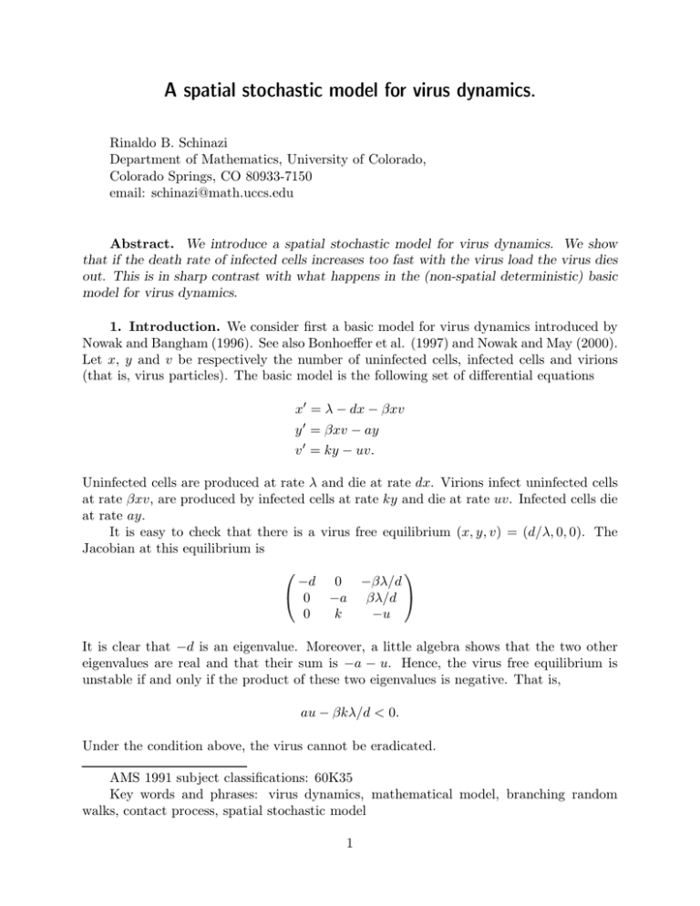
(that is, virus particles). The basic model is the following set of differential equations
x0 = λ − dx − βxv
y 0 = βxv − ay
v 0 = ky − uv.
Uninfected cells are produced at rate λ and die at rate dx. Virions infect uninfected cells
at rate βxv, are produced by infected cells at rate ky and die at rate uv. Infected cells die
at rate ay.
It is easy to check that there is a virus free equilibrium (x, y, v) = (d/λ, 0, 0). The
Jacobian at this equilibrium is

−d
 0
0
0
−a
k

−βλ/d
βλ/d 
−u
It is clear that −d is an eigenvalue. Moreover, a little algebra shows that the two other
eigenvalues are real and that their sum is −a − u. Hence, the virus free equilibrium is
unstable if and only if the product of these two eigenvalues is negative. That is,
au − βkλ/d < 0.
Under the condition above, the virus cannot be eradicated.
AMS 1991 subject classifications: 60K35
Key words and phrases: virus dynamics, mathematical model, branching random
walks, contact process, spatial stochastic model
1
A natural generalization of this model is to let a be a function of v instead of being
a constant. If the death rate of infected cells increases too fast with the viral load (that
is, the number of virions) the virus should not be able to establish itself. In order to test
this idea, consider an increasing continuous function a such that a(0) > 0. Consider the
system above with the only difference that a is now a function of v. We have the same
virus free equilibrium as before and the Jacobian is the same as before except that a is
replaced by a(0). Hence, the virus free equilibrium is unstable if and only if
d
k
a(0) − λ < 0.
β
u
This condition does not depend on the shape of the function a and even if a increases very
fast the virus free equilibrium is still unstable. Next we introduce a model whose behavior
is drastically different.
2. The spatial stochastic model. The new model evolves on the square lattice Zd ,
typically d = 2 but our results hold in any dimension d ≥ 1. At each site x in the square
lattice Zd there may be a cell and up to N virions. We denote our stochastic process by
ηt . For a site x in Zd we set ηt (x) = (i, v) where i is 0 or 1 and v is an integer between
0 and N . The first coordinate i indicates whether a cell is present at x (i = 1 indicates
the presence of a cell, i = 0 indicates the absence of a cell) and the second coordinate v
counts the number of virions at site x. Thus, we are assuming that there is a maximum of
one cell and of N virions at a given site. In what follows, the parameter N can be taken
arbitrarily large.
We first describe the model informally. Cells are produced at a constant rate λ. The
death rate of a cell is a(v) where v is the number of virions present at the same site, v is
an integer in {0, 1 . . . N }. Virions replicate at rate k if a cell is present at the same site. A
virus jumps to a neighboring site at rate β, this is how the infection spreads in this model.
The jump is allowed only if the neighboring site has not reached the maximal viral load
N . A virus dies at a constant rate u. We assume that a is a continuous and increasing
function with a(0) > 0.
We now give a more formal description. Let nv (x, η) be the total number of virions
in the 2d nearest neighbors of site x when the model is in configuration η. Let nN (x, η)
be the number of nearest neighbor sites of x in state (i, N ) where i = 0 or 1. That is,
nN (x, η) is the number of nearest neighbors of site x that have reached the maximal virus
load N . Assume that the model is in configuration η then the state at a given site x
changes according to the following transition rates:
(0, v) → (1, v) at rate λ for 0 ≤ v ≤ N
(0, v) → (0, v + 1) at rate βnv (x, η) for 0 ≤ v ≤ N − 1
(1, v) → (0, v) at rate a(v) for 0 ≤ v ≤ N
(1, v) → (1, v + 1) at rate k + βnv (x, η) for 1 ≤ v ≤ N − 1
(1, 0) → (1, 1) at rate βnv (x, η)
(i, v) → (i, v − 1) at rate uv + β(2d − nN (x, η))v for 1 ≤ v ≤ N and i = 0, 1
2
The last transition keeps track of the two ways of losing a virus at site x: either by death
(at rate u) or if the virus jumps to one of the 2d neighboring sites (at rate β) that has not
yet reached its maximal viral load N .
We say that the virus dies out if for any initial configuration and any fixed site x in
d
Z there is, with probability 1, a random time after which there will never be a virion at
x. We say that the virus survives if there is at least one initial configuration for which
there is a positive probability that at all times there will be at least one virion somewhere
in Zd .
We are ready to state our first and main result.
Theorem 1. Consider the spatial stochastic model with parameters β > 0, u ≥ 0,
N ≥ 2 and a(v) = c + bv p with c > 0 and p > 0. There is B (depending on β, u, N , c, b
and p) such that if b > B then the virus dies out.
In words, the virus cannot survive if the function a grows too fast. This is in sharp
contrast with the behavior of the basic model for which the condition of survival of the
virus depends only on a(0). As the reader will be able to check, our proof works for a
much larger class of functions a than the one stated in Theorem 1.
Our second result is that if λ and k are both large then the virus may survive.
Theorem 2. Consider the spatial stochastic model with fixed values for parameters
β > 0, u ≥ 0 and N ≥ 2 and with an increasing function a such that a(0) > 0. There are
numbers K and Λ (both depending on β, u, N and a) such that for k > K and λ > Λ the
virus survives.
The preceding result shows that the virus may survive if λ and k are both large
enough. Next we show that if k or λ are too low the virus cannot survive.
Theorem 3. Consider the spatial stochastic model with fixed values for parameters
β > 0, u ≥ 0 and N ≥ 2 and with an increasing function a such that a(0) > 0.
(i) For any given k there is ` > 0 such that if λ < ` the virus dies out.
(ii) For any given λ there is κ > 0 such that if k < κ the virus dies out.
We show in Theorem 1 that if a(v) = c + bv p and if b is too large (i.e. the death rate of
infected cells increases too fast with the virus load) then the virus cannot establish itself.
Contrary to what happens in the basic model a virion infects only nearby cells so if the
cells die too fast the virus runs out of fuel and dies out. In the basic model the virions are
mixed to all the cells, giving it more opportunities for infection even if the cost of infection
is very high (i.e. very high death rate for infected cells). We believe it is the introduction
of space and the localization of the infection that causes the crucial difference in behavior
between the two models. A similar result was proved in Schinazi (2003).
In the mathematical biology literature there is interest in understanding why some
viruses, such as HIV, are not eradicated, even under successful treatment (see 4.2.6 in
Nowak and May (2000)). One hypothesis is that ’long lived cells’ continue to produce
virions for a long time. Another possible explanation, suggested by our results, is that
whether a virus is eradicated depends on the virus dynamics. If the dynamics is global
such as in the basic model then eradication is not possible. If the dynamics is local such
as in the spatial model then eradication is possible.
3
In theorem 2 we show that if the birth rate of healthy cells and the replication rate of
virions are large enough then the virus may establish itself. In Theorem 3 we show that
if one of these two rates drops too low then the virus dies out. Theorem 3 (i) suggests
a strategy for the immune system to fight a virus. If the birth rate of healthy cells is
too low (or, equivalently, if the death rate of healthy cells is too high) then the virus
cannot establish itself. This is consistent with the recent observation that most of the T
cell destruction associated with HIV infection involves healthy cells, see Hellerstein et al.
(2003) and Silvestri and Feinberg (2003).
As for all models, our models have their limitations. Some viruses (such as HIV) are
successful because of their high mutation rates (see for instance, Nowak and May (2000)).
The present models do not include mutation. Another assumption that we make and may
or may not apply (depending on the type of virus) is that cells do not reproduce locally.
This applies, for instance, to T cells that are produced in the bone marrow (and are the
target of HIV virus). Finally, it is also possible that, contrary to what we assume, some
viruses inhibit further infection of an infected cell.
3. Proofs.
Construction of the spatial stochastic process
We use the so called graphical construction that was first introduced by Harris (1972).
All the different Poisson processes that we will now introduce are independent.
At each site x of Zd , let (dxm )m≥1 be a sequence of independent identical Poisson
processes with rate u. The mth virion appearing at site x is labeled m. At the arrival
times of the Poisson process dxm we kill virion m if it is at x. That is, the state at site x
jumps from (i, v) to (i, v − 1). At each site x, we also have a Poisson process bx with rate
k. At arrival times of bx the state at x jumps from (i, v) to (i, v + 1) if i = 1 (i.e. there is
a cell at x) and if 1 ≤ v ≤ N − 1 (i.e. the cell is already infected but has not reached its
maximum virus load). For each ordered pair of neighboring sites x, y we have a sequence
x,y
(Im
)m≥1 of independent identical Poisson processes with rate β. At the arrival times of
x,y
Im , if virion m is at x it jumps to y if the viral load at y is less than N . That is, the state
at x jumps from (i, v) to (i, v − 1) and simultaneously the state at y jumps from (i, v) to
(i, v + 1) for i = 0 or 1. We also use Poisson processes for birth and death of cells. At
each site x we have two independent Poisson processes B x and D x with rates λ and a(N ),
respectively. At the arrival times of B x the state of x jumps from (i, v) to (1, v) (nothing
happens if i = 1). At the arrival times of D x the state of x jumps from (i, v) to (0, v) with
probability a(v)/a(N ) (recall that a is an increasing function). Thus, nothing happens if
i = 0 and it is easy to see that with this recipe (1, v) jumps to (0, v) at rate a(v).
It is not difficult to see that this construction provides the spatial stochastic process
with the prescribed rates. In what follows we will also need to consider the process restricted
to a space time box B = (−4L, 4L)d × [0, T ]. In order to construct the restricted process
we use the same Poisson processes as above but only for sites in (−4L, 4L)d and up to
time T .
For the construction of a similar process see Pemantle and Stacey (2001). For more
on graphical constructions, see Durrett (1995).
Proofs of Theorems 1 and 3.
4
We will first deal with the proof of Theorem 1 and then explain how to adapt it to
Theorem 3. We write the proof in dimension d = 2. The same ideas work in any d ≥ 1.
We start by defining two space-time regions.
A = [−2L, 2L]2 × [0, 2T ]
B = [−L, L]2 × [T, 2T ].
Note that B is nested in A. Let C be the boundary of A:
C = {(m, n, t) ∈ A : |m| = 2L or |n| = 2L or t = 0}.
We will compare the process ηt to a percolation process on Z2 × Z+ . We declare
(k, m, n) in Z2 × Z+ wet if for the process restricted to A + (k, m, n) there is no virion in
B +(k, m, n). Moreover, we want no virion in B +(k, m, n) for any possible configuration of
the boundary C + (k, m, n). In particular, this must be true even if all sites in C + (k, m, n)
are in state (1, N ).
Recall that a(v) = c + bv p . We start by setting b = ∞ in A. This means that a(0) = c
and a(v) = ∞ for v ≥ 1, as soon as a virion lands on a cell it kills it. There can be
no creation of virion in A. The virions inside A must all come from the boundary C. A
virion that makes it into B must either have originated in [−2L, 2L] × {0} or at a later
time from one of the sides of box A. In the former case the virion must have survived at
least T before it reaches B while in the latter case it must have traveled at least L inside
A. Note that a virion in A under condition b = ∞ performs a random walk and has a
constant death rate u. The probability that a virion survives longer than T units of time
is therefore exp(−uT ). In order for a virion to travel L units of space or more it must
either survive L/(2β) units of time or it must travel L in less than L/(2β) units of time.
Note that the total advance up to time L/(2β) along one coordinate for a given virion is
a Poisson random variable with mean L/2. Let X be such a random variable. Using the
Chebyshev’s exponential inequality we have
P (X > L) ≤ exp(−θL)E(exp(θX)) = exp(−θL) exp(−L/2) exp(eθ L/2)
for any θ > 0. Letting θ = ln 2 in the inequality above yields
P (X > L) ≤ exp(L(− ln 2 + 1/2))
which converges to 0 exponentially fast as L goes to infinity. Putting together the preceding
estimates and using that there are at most N virions on each site of the boundary C we
get
(1)
P ((0, 0, 0) is wet) ≥ 1 − N (4L + 1)2 e−uT − N 8L(4L + 1) exp(L(− ln 2 + 1/2)).
For any > 0 there are T = L such that
P ((0, 0, 0) is wet) ≥ 1 − /2 for b = ∞.
We now deal with finite b. Consider the following event. For each site x in [−2L, 2L]2 and
up to time 2T every time a virion lands on x there is a death of the cell at x (with rate
5
c + b) before the virion is replicated (with rate k). Since we are dealing with finitely many
sites and a finite time, by taking B much larger than k we have that the preceding event
happens with probability 1 − /2 provided b > B. In particular,
P ((0, 0, 0) is wet) ≥ 1 − for b > B.
By translation invariance, the same is true for any site (k, m, n) of Z2 × Z+ .
Note that the event ’(k, m, n) is wet’ depends only on the Poisson processes inside
A + (k, m, n). This allows us to define a percolation process on Z2 × Z+ with finite range
dependence. A dry (i.e. not wet) site has probability in this percolation process, see the
proof of Theorem 4.4 in Berg et al. (1998) for more details. If there is a virion somewhere
at some time for the process ηt then there must be a path of dry sites in the percolation
process. Moreover, by taking > 0 small enough one can make the probability of a path
of dry sites of length n decrease exponentially fast with n. This, in turn implies that for
any given site there will be no virion after a finite random time, see (8.2) in Berg et al.
(1998). This completes the proof of Theorem 1.
For Theorem 3 (i) we use the construction above with λ = 0 in box A. Using that a
is an increasing function of v, all the cells in A are dead by time T /2 with probability at
least
2
(1 − e−a(0)T /2 )(4L+1) .
The probability above can be made arbitrarily close to 1 provided T = L are large enough.
Given that all the cells are dead the virions in box A cannot replicate. They can only
perform random walks until they die. The same estimates as in (1) may be adapted to
this case (we only need to replace T by T /2 in (1)) to show that the probability that no
virion lands in box B can be made as close to 1 as we want. We then argue that since A is
a finite space time box this event has a probability close to 1 if λ < ` where ` > 0 is small
enough. The rest of the proof is the same.
The proof of Theorem 3 (ii) is even easier since if we take k = 0 in A a virion cannot
replicate in A. So estimate (1) holds in this case with no modification.
Proof of Theorem 2.
We write the proof in dimension 2 to avoid more cumbersome notation. Let e1 be the
vector (1, 0) and
L = {(m, n) ∈ Z2 : m + n is even}
B = (−4L, 4L)2 × [0, T ]
I = [−L, L]2
Bm,n = (2mLe1 , nT ) + B
Im = 2mLe1 + I
where L and T are parameters to be chosen later. We declare (m, n) ∈ L wet if the process
restricted to Bm,n and starting at time nT with at least one site in Im in state (1, N ) is
such that there is at least one site in Im−1 and in Im+1 in state (1, N ). In other words,
we declare (m, m) wet if a site in state (1, N ) at time nT is duplicated at time (n + 1)T in
Im−1 and in Im+1 .
We will now show that by choosing L and T sufficiently large the probability of a site
(m, n) being wet can be made arbitrarily close to 1. By translation invariance, it is enough
6
to show this for the site (0,0). We start by setting k = ∞ and λ = ∞ in the box B. This
means that as soon as a cell dies it is replaced and that as soon as there is a virion on
a cell the virus load increases to its maximum load N . Under these conditions there are
only two possible states for each site: (1, 0) and (1, N ). Moreover, once a site is in state
(1, N ) it stays in that state: as soon as a virion dies or jumps to a neighboring site it is
replaced since k = ∞.
Assume that at time 0 there is at least one site of I in state (1, N ). So there is a site
with coordinates (i, j), −L ≤ i ≤ L and −L ≤ j ≤ L, in state (1, N ) at time 0. After an
exponential time with rate N β a virion jumps from site (i, j) to site (i + 1, j) and this site
is now in state (1, N ). After another (and independent) exponential time with rate N β a
virion jumps from site (i + 1, j) to site (i + 2, j) and this site is now in state (1, N ), and so
on. Thus, the rightmost site in state (1, N ) on the segment (x, j), for i ≤ x ≤ 2L, advances
at least like a Poisson process with rate N β. The fact that this process is actually on a
multidimensional space will make the rightmost site advance more quickly (but no faster
than linearly). By the Law of Large Numbers, for any > 0, if L is large enough then
7L
by time T = 2N
β all the sites (x, j), for i ≤ x ≤ 2L, are in state (1, N ) with probability
at least /4. Symmetrically, by time T all the sites (x, j), for −2L ≤ x ≤ i, are in state
7L
(1, N ) with probability at least /4. This shows that for any > 0 we may pick T = 2N
β
and L large enough so that
P ((0, 0) is wet) > 1 − /2 for λ = ∞ and k = ∞.
We now show that k and λ may be taken finite. The process restricted to B with finite
k and λ will have the same behavior as the process with infinite λ and k if the following
events happen. Every time there is a death of a cell at a given site (with maximum rate
a(N )) we want a birth of a cell (with rate λ) to happen before any death of virion (with
maximum rate uN ). If a site is in state (1, v) with 1 ≤ v ≤ N − 1 we want it to jump to
state (1, v + 1) (with rate k) before a virion or the cell dies (with rate a(v) + uv). Since we
are dealing with finitely many sites and finite time, by taking λ and k much larger than
a(N ) + uN the preceding event will have a probability at least 1 − /2. Thus, for any > 0
there are Λ and K depending on β, N , u and a such that
P ((0, 0) is wet) > 1 − for λ > Λ and k > K.
The rest of the proof is pretty standard and we only outline it. A crucial ingredient
is that the event ’(m, n) is wet’ only depends on Poisson processes inside the box Bm,n .
Therefore, if |m − j| > 1 or |n − k| > 1 the events ’(m, n) is wet’ and ’(j, k) is wet’ are
independent. This implies for > 0 small enough that there is percolation of wet sites,
see for instance Theorem A.1. in Durrett (1995). This in turn implies that virions survive
forever.
Acknwoledgements. We thank a referee for remarks that helped improve the paper.
References.
7
J. van den Berg, G. Grimmett and R. Schinazi (1998). Dependent random graphs
and spatial epidemics. Annals of Applied Probability 8, 317-336.
S.Bonhoeffer, R.M.May, G.M.Shaw and M.A.Nowak (1997). Virus dynamics and drug
therapy. Proc. Natl. Acad. Sci., Vol. 94, 6971-6976.
R. Durrett (1995). Ten lectures on particle systems. Lecture notes in Mathematics,
Vol. 1608, Springer-Verlag, New York.
T.Harris (1972). Nearest neighbor interaction processes on multidimensional lattices.
Adv. Math. 9, 66-89.
M.K.Hellerstein et al. (2003). Subpopulations of long-lived and short-lived T cells in
advanced HIV-1 infection. The Journal of Clinical investigation, 112, 956-966.
T.M.Liggett (1985). Interacting particle systems. Springer-Verlag, New York.
M.A.Nowak and C.R.M. Bangham (1996). Population dynamics of immune responses
to persistent viruses. Science, Vol. 272, 74-79.
M.A.Nowak and R.M. May (2000). Virus Dynamics: Mathematical Principles of
Immunology and Virology. Oxford University Press.
R. Pemantle and A. M. Stacey (2001). The Branching Random Walk and Contact
Process on Galton-Watson and Nonhomogeneous Trees. Ann. Probab. 29, 1563-1590.
R.B.Schinazi (2003). On the role of reinfection in the transmission of infectious diseases. Journal of Theoretical Biology, 225, 59-63.
G. Silvestri and M.B.Feinberg (2003). Turnover of lymphocytes and conceptual paradigms in HIV infection. The Journal of Clinical investigation, 112, 821-824.
8