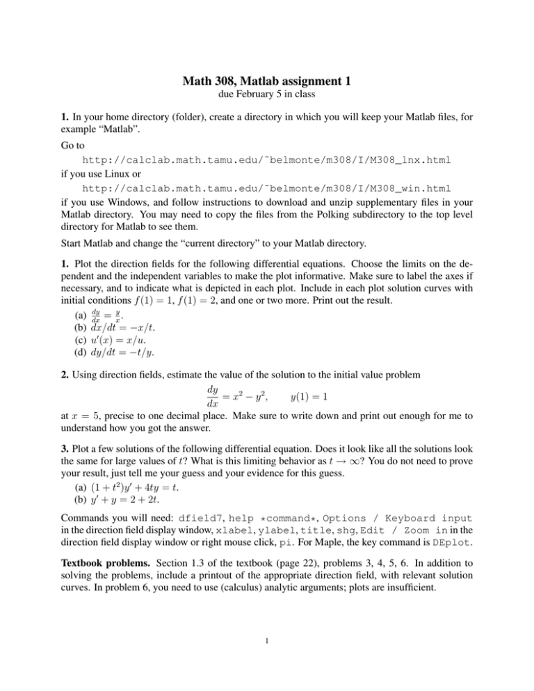
Math 308, Matlab assignment 1
due February 5 in class
1. In your home directory (folder), create a directory in which you will keep your Matlab files, for
example “Matlab”.
Go to
http://calclab.math.tamu.edu/˜belmonte/m308/I/M308_lnx.html
if you use Linux or
http://calclab.math.tamu.edu/˜belmonte/m308/I/M308_win.html
if you use Windows, and follow instructions to download and unzip supplementary files in your
Matlab directory. You may need to copy the files from the Polking subdirectory to the top level
directory for Matlab to see them.
Start Matlab and change the “current directory” to your Matlab directory.
1. Plot the direction fields for the following differential equations. Choose the limits on the dependent and the independent variables to make the plot informative. Make sure to label the axes if
necessary, and to indicate what is depicted in each plot. Include in each plot solution curves with
initial conditions f (1) = 1, f (1) = 2, and one or two more. Print out the result.
dy
= xy .
(a) dx
(b) dx/dt = −x/t.
(c) u0 (x) = x/u.
(d) dy/dt = −t/y.
2. Using direction fields, estimate the value of the solution to the initial value problem
dy
= x2 − y 2 ,
y(1) = 1
dx
at x = 5, precise to one decimal place. Make sure to write down and print out enough for me to
understand how you got the answer.
3. Plot a few solutions of the following differential equation. Does it look like all the solutions look
the same for large values of t? What is this limiting behavior as t → ∞? You do not need to prove
your result, just tell me your guess and your evidence for this guess.
(a) (1 + t2 )y 0 + 4ty = t.
(b) y 0 + y = 2 + 2t.
Commands you will need: dfield7, help *command*, Options / Keyboard input
in the direction field display window, xlabel, ylabel, title, shg, Edit / Zoom in in the
direction field display window or right mouse click, pi. For Maple, the key command is DEplot.
Textbook problems. Section 1.3 of the textbook (page 22), problems 3, 4, 5, 6. In addition to
solving the problems, include a printout of the appropriate direction field, with relevant solution
curves. In problem 6, you need to use (calculus) analytic arguments; plots are insufficient.
1