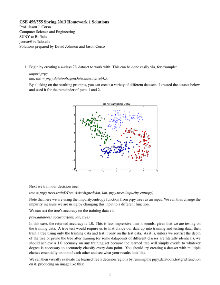
CSE 455/555 Spring 2013 Homework 1 Solutions
Prof. Jason J. Corso
Computer Science and Engineering
SUNY at Buffalo
jcorso@buffalo.edu
Solutions prepared by David Johnson and Jason Corso
1. Begin by creating a 4-class 2D dataset to work with. This can be done easily via, for example:
import prpy
dat, lab = prpy.datatools.genData interactive(4,5)
By clicking on the resulting prompts, you can create a variety of different datasets. I created the dataset below,
and used it for the remainder of parts 1 and 2.
Done Sampling Data
10
8
6
4
2
0
−2
−4−6
−4
−2
0
2
4
6
Next we train our decision tree:
tree = prpy.trees.trainDTree AxisAligned(dat, lab, prpy.trees.impurity entropy)
Note that here we are using the impurity entropy function from prpy.trees as an input. We can thus change the
impurity measure we are using by changing this input to a different function.
We can test the tree’s accuracy on the training data via:
prpy.datatools.accuracy(dat, lab, tree)
In this case, the returned accuracy is 1.0. This is less impressive than it sounds, given that we are testing on
the training data. A true test would require us to first divide our data up into training and testing data, then
train a tree using only the training data and test it only on the test data. As it is, unless we restrict the depth
of the tree or prune the tree after training (or some datapoints of different classes are literally identical), we
should achieve a 1.0 accuracy on any training set because the learned tree will simply overfit to whatever
degree is neccesary to accurately classify every data point. You should try creating a dataset with multiple
classes essentially on top of each other and see what your results look like.
We can then visually evaluate the learned tree’s decision regions by running the prpy.datatools.testgrid function
on it, producing an image like this:
1
10
5
0
−5
−10
−10
−5
0
5
10
We probably aren’t seeing all the finer detail because of the scale of the grid used here, but one thing to note
here is how the tree, because the splitting functions it uses are axis aligned, divided the data up using only a
succession of straight horizontal and vertical cuts.
2. The impurity gini method can be written quite easily by copying the impurity entropy method and changing
a few lines of code:
def impurity_gini(Y):
’’’ Calculate the Gini impurity for a data set (Y). ’’’
U = np.unique(Y)
imp = 1
for c in U:
yc = np.nonzero(Y==c)[0]
# like matlab’s find()
if (len(yc)==0):
continue
cportion = len(yc)/np.double(len(Y))
imp -= cportion**2
return imp
This change will probably only produce minor differences in your results (as visualized by the testgrid
method), although it did cause one of the leaf nodes for my example data to reach the depth limit allowed
in this code. The node was thus not totally pure, leading to a not-quite-perfect classification result (0.9975
accuracy) on the training data.
3. A completed version of the rfdigits file can be found at http://www.cse.buffalo.edu/˜jcorso/
t/CSE555/files/rfdigits.py. Those who are interested should feel free to experiment with this
code—just be sure to change the “kMNIST PATH” variable to point to wherever you have stored the MNIST
data and run the script using “python rfdigits.py”.
2
For reference, my test run returned a 1.0 accuracy on the training data and an 0.685 accuracy on the test data.
You may wish to try different parameters or even alter the algorithm in order to get a higher score. It should
be possible to achieve a score in the high 90% range using random forests, though that will likely require
learning a larger forest and doing a more exhaustive search of the features than this code does by default, and
will likely be quite slow, given that this code is written for readability rather than efficiency.
3