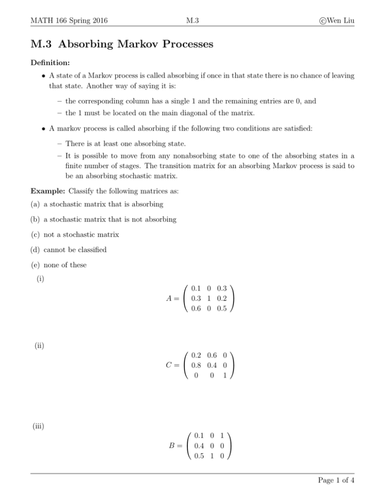
MATH 166 Spring 2016
M.3
c
Wen
Liu
M.3 Absorbing Markov Processes
Definition:
• A state of a Markov process is called absorbing if once in that state there is no chance of leaving
that state. Another way of saying it is:
– the corresponding column has a single 1 and the remaining entries are 0, and
– the 1 must be located on the main diagonal of the matrix.
• A markov process is called absorbing if the following two conditions are satisfied:
– There is at least one absorbing state.
– It is possible to move from any nonabsorbing state to one of the absorbing states in a
finite number of stages. The transition matrix for an absorbing Markov process is said to
be an absorbing stochastic matrix.
Example: Classify the following matrices as:
(a) a stochastic matrix that is absorbing
(b) a stochastic matrix that is not absorbing
(c) not a stochastic matrix
(d) cannot be classified
(e) none of these
(i)


0.1 0 0.3
A =  0.3 1 0.2 
0.6 0 0.5
(ii)


0.2 0.6 0
C =  0.8 0.4 0 
0
0 1
(iii)


0.1 0 1
B =  0.4 0 0 
0.5 1 0
Page 1 of 4
MATH 166 Spring 2016
c
Wen
Liu
M.3
Theorem 1: In an absorbing Markov process, the long term probability of going from any nonabsorbing state to some absorbing state is one.
Theorem 2: Let T be the transition matrix of an absorbing Markov process with a absorbing states
and b nonabsorbing states. Reorder the states so that the first a of them are absorbing and the
remaining b of them are nonabsorbing. Partition the matrix as follows
A=
Absorbing
Nonabsorbing
Absorbing
Nonabsorbing
Ia×a
Ob×a
Aa×b
Bb×b
Then the following is true.
• As n becomes large without bound, the matrix T n , which is the transition matrix from the
initial stage to the nth stage, heads for the limiting matrix
"
#
Ia×a A(I − B)−1
L=
Ob×a
Ob×b
where the identity matrix, I, in the expression (I − B)−1 is the same dimension as B, that is,
b × b.
• The entry in the ith row and jth column of the sub-matrix A(I − B)−1 gives the probability
that the system will end up in the ith absorbing state when initially in the jth nonabsorbing
state.
• All column sums of A(I − B)−1 are 1, and thus everything is expected to be absorbed.
Examples:
1. In the Estes learning model it is assumed a person is in state 1 if he has learned a particular
task and state 2 if he has not. Once a person learns a task, he never forgets it. If a person has
not learned the task, there is a probability of 0.15 that he will learn it during the next time
period.
(a) Write the transition matrix.
(b) What is the long term behavior? More precisely, what is the probability the person has
learned the task? What is probability the person has not learned the task?
Page 2 of 4
MATH 166 Spring 2016
c
Wen
Liu
M.3
2. The following matrix is a transition matrix for an absorbing Markov process. Find the limiting
matrix.


1 0 0.25 0.1


 0 1 0.25 0.25 
X=

 0 0 0.2 0.1 
0 0 0.3 0.55
3. A certain manufacturing process consists of 2 manufacturing states (1 and 2) and a completion
state (C) together with a fourth state in which the item is scrapped if improperly manufactured
(S). At the end of each of the 2 manufacturing states each item is inspected. At each inspection
there is a probability of 0.35 that the item will be passed on to the next state (the first
manufacturing state to the second or the second manufacturing state to the completion state),
probability of 0.15 that it will be sent back to the same state for reworking, and probability of
0.5 that the item will be scrapped. Naturally, an item that is complete stays complete, and an
item that is scrapped stays scrapped.
(a) Write a transition matrix for this Markov process.
(b) Determine the long-term behavior.
The probability for the item to go from
The probability for the item to go from
The probability for the item to go from
The probability for the item to go from
state
state
state
state
1
1
2
2
to
to
to
to
scrapped is:
completion is:
scrapped is:
completion is:
Page 3 of 4
MATH 166 Spring 2016
c
Wen
Liu
M.3
4. A credit card account is classified at the end of each month as “paid,” “overdue less than 30
days,” “overdue less than 60 days,” or “overdue 60 days or more.” In the last case, the debt is
judged “bad” and the account is closed. Each month the debt can age by at most one month,
keep the same or lesser age by means of a payment, or be paid off. If paid off, the account
remains paid off. Over a period of time the company has obtained figures that give the following
transition matrix.
Paid < 30 < 60 Bad


Paid
1
0.3
0.12
0
< 30  0
0.22 0.35
0


< 60  0
0.48 0.32
0
Bad
0
0
0.21
1
Determine the long-term behavior.
probability that an account classified
probability that an account classified
probability that an account classified
probability that an account classified
as
as
as
as
< 30
< 30
< 60
< 60
will
will
will
will
be
be
be
be
ultimately
ultimately
ultimately
ultimately
classified
classified
classified
classified
as
as
as
as
Paid:
Bad:
Paid:
Bad:
Page 4 of 4