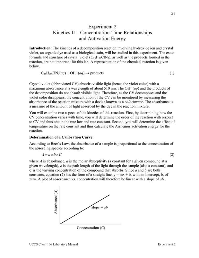
2-1
Experiment 2
Kinetics II – Concentration-Time Relationships
and Activation Energy
Introduction: The kinetics of a decomposition reaction involving hydroxide ion and crystal
violet, an organic dye used as a biological stain, will be studied in this experiment. The exact
formula and structure of crystal violet (C25H30ClN3), as well as the products formed in the
reaction, are not important for this lab. A representation of the chemical reaction is given
below.
C25H30ClN3(aq) + OH– (aq) → products
(1)
Crystal violet (abbreviated CV) absorbs visible light (hence the violet color) with a
maximum absorbance at a wavelength of about 510 nm. The OH– (aq) and the products of
the decomposition do not absorb visible light. Therefore, as the CV decomposes and the
violet color disappears, the concentration of the CV can be monitored by measuring the
absorbance of the reaction mixture with a device known as a colorimeter. The absorbance is
a measure of the amount of light absorbed by the dye in the reaction mixture.
You will examine two aspects of the kinetics of this reaction. First, by determining how the
CV concentration varies with time, you will determine the order of the reaction with respect
to CV and thus obtain the rate law and rate constant. Second, you will determine the effect of
temperature on the rate constant and thus calculate the Arrhenius activation energy for the
reaction.
Determination of a Calibration Curve:
According to Beer’s Law, the absorbance of a sample is proportional to the concentration of
the absorbing species according to:
A = a×b×C
(2)
Absorbance (A)
where A is absorbance, a is the molar absorptivity (a constant for a given compound at a
given wavelength), b is the path length of the light through the sample (also a constant), and
C is the varying concentration of the compound that absorbs. Since a and b are both
constants, equation (2) has the form of a straight line, y = mx + b, with an intercept, b, of
zero. A plot of absorbance vs. concentration will therefore be linear with a slope of ab.
slope = ab
Concentration (C)
UCCS Chem 106 Laboratory Manual
Experiment 2
2-2
By measuring the absorbance of solutions of CV with known concentration, a calibration
curve can be prepared. Using the equation of the line for the calibration curve, any
concentration of CV can be determined from the measured absorbance of the solution.
The colorimeter actually measures how much light is transmitted through the sample. The
transmittance is defined as the fraction of the incident light that passes through the sample
and reaches the detector. In this experiment, the Vernier colorimeter will automatically
convert the transmittance to absorbance (a dimensionless quantity).
Determination of the Order of the Reactant CV:
The rate expression for reaction (1) is:
Rate = k[CV]m [OH - ]
(3)
where k is the rate constant of the reaction and m is the order of the reaction with respect to
CV. It is known that the order of the reaction with respect to the OH− ion is 1. Analysis of the
kinetics can be greatly simplified by keeping the hydroxide concentration much larger than
the concentration of the crystal violet, [OH–] >> [CV]. When this is done, so little OH– is
consumed compared to the initial high concentration of hydroxide, that [OH–] remains
virtually constant throughout the course of the reaction. This allows for a modified
expression for the rate law:
Rate = k[OH - ][CV]m = k ′[CV]m
with k′ = k[OH–]
(4)
The constant k′ is called a pseudo rate constant because it is a constant that relates the
reaction rate to [CV]m , but only provided that [OH–] remains constant. Note that k′ would
have a different value for a different [OH–].
In order to determine the value of m, you will measure the absorbance of the reaction mixture
as a function of time. Once the absorbance (and hence [CV]) has been measured as a function
of time, it is possible to determine the reaction order from the relationship between [CV] and
time. For zero, first and second order reactions, there are different concentration-time
relationships derived using calculus. The resulting equations are discussed in your textbook
and class notes and are summarized in Table 1 (page 2-3).
Therefore to determine the order, m, of the reactant CV from your [CV] vs. time data,
you will create three plots, [CV] vs. time, ln[CV] vs. time, and 1/[CV] vs. time. The plot
that gives a straight line for your data determines the reaction order as indicated in Table 1.
Furthermore, the absolute value of the slope of the linear plot equals the pseudo rate
constant, k′, which always has a positive value. (Note that measured slope is either positive
or negative, and that the units of the slope differ, as indicated in Table 1). Also since the
known order for [OH−] is n=1, from equation (4), we get
k=
k'
[OH − ]
UCCS Chem 106 Laboratory Manual
(5)
Experiment 2
2-3
which allows calculation of the rate constant, k, from the pseudo rate constant, k′, obtained
as the slope and the known value of [OH−] for the reaction mixture.
Order with
respect to R
Rate Expression and ConcentrationTime Relationship
Graph
Slope
k′ units
Zero, n = 0
[R]t = –k′t + [R]0
[R] vs. t
– k′
M s-1
First, n = 1
ln[R]t = –k′t + ln[R]0
ln[R] vs. t
– k′
s-1
Second, n = 2
1/[R]t = k′t + 1/[R]0
1/[R] vs. t
k′
M-1 s-1
Table 1. A summary of concentration-time relationships for pseudo- zero, first and second
order rate laws. [R] represents the concentration of the reactant, CV, in the rate law. Note
that although the slope may be negative, k’ is always positive.
Determination of the Energy of Activation for the Reaction:
The value of the rate constant, k, is constant only for a single temperature. The values of k at
different temperatures are related by the Arrhenius equation,
k = A e - Ea / RT
(6)
−1
−1
where T is temperature in Kelvin; R is the universal gas constant, 8.3145 J mol K ; Ea is
the activation energy of the reaction in J·mol−1; and A is a proportionality constant called the
Arrhenius pre-factor (don’t confuse this with absorbance!). Taking the natural logarithm of
both sides of equation (6) results in the following expressions:
⎛ − Ea ⎞
ln k = ln A + ⎜
⎟ , which can be written as:
⎝ RT ⎠
⎛E
ln k = −⎜ a
⎝ R
⎞⎛ 1 ⎞
⎟⎜ ⎟ + ln A
⎠⎝ T ⎠
(7)
Since –(Ea/R) and ln A are constant, this has the form of a straight line. Thus a plot of lnk vs.
1/T will yield a slope equal to –(Ea/R), allowing calculation of Ea. However if data is
collected at only two temperatures, T1 and T2, the activation energy can be found
algebraically by writing equation (7) twice, substituting once with k1 and T1 and again with k2
and T2. Since the term, ln A, is constant, subtracting the two equations results in:
⎛k ⎞
⎛E
ln⎜⎜ 2 ⎟⎟ = −⎜ a
⎝ R
⎝ k1 ⎠
⎞⎛ 1 1 ⎞
⎟⎜⎜ − ⎟⎟
⎠⎝ T2 T1 ⎠
UCCS Chem 106 Laboratory Manual
(8)
Experiment 2
2-4
Note that the two different reaction temperatures (which must be expressed in degrees
Kelvin, K) will each have a different value of k.
In this experiment the reaction will be done at room temperature and at ~1oC to find two
different values of k′. Then equation (5) will be used to evaluate k at each temperature.
Equation (8) will then be used to determine the activation energy of the reaction.
Pre-Lab Notebook: Provide a title, purpose, reaction(s), summary of the procedure, and a
table of reagents like the one below.
Table of Physical Properties of Chemicals Used:
Compound
Formula Mass, FM (g/mol) Hazards
Crystal violet
Sodium hydroxide
Create a Standard Solutions Table similar to the one in step 7 of Part A and fill in the
values of CV concentration for every flask prior to the start of lab. Use the molarity,
2.5x10−5 M, and volumes of the CV stock solution in flasks B-F given in the Standard
Solutions Table to calculate concentrations in the flasks after dilution to 50.0 mL with DI
water. Note that the molarities of the standard solutions, B-F, will be given by
[CV] = (2.5x10−5 M)(volume in L of CV stock solution)/0.0500L
since each standard solution will have a total volume of 50.0mL.
Equipment:
150 mL Beakers (2)
100 mL Beakers (3)
600 mL Beaker for waste
400 mL Beaker for CV stock solution
Buret
100 mL Graduated cylinder
10 mL Graduated pipet
Disposable pipets
50 mL Volumetric flasks (5)
Ice-Water Bath
Stopwatch
Vernier LabPro
Vernier Colorimeter and cuvettes
Vernier Temperature Probe
TI-84 Calculator
Stock Solutions:
2.5 × 10–5 M Crystal Violet (0.020 g in 2.0 L)
0.40 M NaOH
Experimental Procedure: Work in pairs. Before beginning, do Step C-2. Also note that
due to possible discoloration of the cuvettes by the CV dye, the cuvette you use should
be rinsed with 3M HCl and then DI water at the start of each of the following parts.
Part A: Determination of the Calibration Curve:
1.
Following the first section of the Vernier tutorial, set up the Vernier system in
DATAMATE with the colorimeter connected to channel 1. Allow the colorimeter to warm
up for at least 5 minutes while the standard solutions are prepared.
UCCS Chem 106 Laboratory Manual
Experiment 2
2-5
2.
3.
4.
5.
6.
7.
Set the wavelength on the colorimeter to 565 nm (indicated by the green light) by
pressing the < > arrows on the colorimeter controls.
Label a 50 mL volumetric flask with one of the standard solution labels “A” through
“F” as instructed by the Lab Instructor. Dispense the volume of the CV stock solution
required (See table in step 7) to form the assigned standard solution directly from the
buret containing the stock solution into your labeled volumetric flask. Carefully fill the
flask to the 50.0 mL mark with de-ionized water. (Solution "A" in the Standard
Solutions Table is the undiluted CV solution).
Cover the flask with a small square of Parafilm and invert a few times to mix
thoroughly. Use different Parafilm for each solution.
Before proceeding, YOU MUST properly calibrate the colorimeter by filling the
cuvette*** with DI water, inserting it in the colorimeter, and pushing the CAL button on
the colorimeter. The red LEDs on the face of the colorimeter will flash several times
and the absorbance will read 0 or .001. Record this value in the Absorbance column for
the DI H2O. If you do not get a value near zero, press CLEAR and try again.
*** Note: the plastic cuvettes have one set of opposite sides with ridges designed
for holding the cuvette, and a clear set of sides through which the light to be
absorbed passes. These clear sides must line up with the arrow inside the
colorimeter. Always put the cuvette in the colorimeter in the correct orientation.
After calibration, remove and empty the cuvette. Using your assigned standard solution,
rinse the cuvette once and then fill the cuvette three-fourths full. (Tip: It is easier to
transfer solution into the cuvette using a disposable pipet than pouring directly from a
volumetric flask.)
Wipe the outside clear sides of the cuvette with a tissue wipe. Place the cuvette inside
the colorimeter (clear sides lined to arrow!) and close the lid. Allow 15 seconds to pass
for the colorimeter to take an accurate reading. When the absorbance reading
stabilizes, record the reading in your Standard Solutions Table and in the table your
Instructor has drawn on the blackboard.
Complete the Standard Solutions Table below by calculating all the CV concentrations
and entering the Absorbance values recorded by other teams:
Flask Volume of Stock CV (mL) Concentration of CV (M) Absorbance
A
50.0
0.000025
B
40.0
C
30.0
D
20.0
E
10.0
F
5.0
DI H2O
0.0
0.0
Part B: Determination of Order of the Reactant CV: (Kinetic Run – Room Temperature)
1.
Set up the Vernier system with the colorimeter connected to channel 1 and the
temperature probe connected to channel 2.
2.
Set the data collection mode on the LabPro: On the main screen of the datamate
program, go to setup and move the cursor until it’s to the left of the mode selection and
press enter. Select “2” for time graph mode. Select change time settings. Type “5” for
UCCS Chem 106 Laboratory Manual
Experiment 2
2-6
3.
the time between samples in seconds, and press enter. Type “100” for the number of
samples, and press enter. Therefore for this run, data will be collected every 5 seconds
for a total of 500 seconds. Select OK twice to return to the main screen.
Using the buret, transfer 20.0 mL of CV stock solution into a 150 mL beaker. Place the
temperature probe into this solution and leave it there for the entire run. Using a 10 mL
graduated pipet, transfer 5.0 mL of 0.40 M NaOH into a 50 mL beaker. The reaction
will not begin until the solutions in the two beakers are mixed.
Add the NaOH to the CV solution and immediately press 2 for START on the calculator.
Swirl the beaker for a 5-10 seconds after mixing to mix well. Rinse and fill the cuvette
¾ full with the mixed solution, wipe the clear sides, and place the cuvette into the
colorimeter.
Once the LabPro beeps, the run is complete, press STO>. In your notebook, note the
shape of the plotted data and then hit ENTER to get out of the graph. Select “6” for QUIT
from the main screen. Then press ENTER on the screen that indicates your data location.
Transfer this data (from L1, L2, and L3) to the Logger Pro computer program. Cut and
paste the columns of data (starting with the first high value for absorbance!) into
Microsoft Excel. Label and save the Excel file for later analysis in the post-lab section.
4.
5.
6.
Part C: Determination of the Energy of Activation for the Reaction: (Kinetic Run ~1°C)
1.
2.
Set up the data collection mode in the DATAMATE program to EVENTS WITH ENTRY
mode. Since the temperature must be constant and close to 1oC, the reaction mixture is
left in the ice-water bath. Using a disposable pipet, samples will be extracted from the
reaction mixture (while it remains in the ice bath) and placed in the cuvette for
absorbance measurements at times measured using a stopwatch. Each absorbance
measurement is an EVENT with the stopwatch time will be recorded as an ENTRY.
Transfer 60 mL of CV stock solution using a 100 mL graduated cylinder into a 150 mL
beaker. Using the graduated pipet, transfer 15.0 mL of 0.40 M NaOH into a separate 50
mL beaker. Place both beakers into an ice-water bath in a clear plastic container. Be
careful that the water level in the ice-bath is not so high as to cause the beakers to turn
over in the bath or water from the bath to seep into the beakers.
To avoid confusion during this experiment, read and understand steps 3-7 before
proceeding! Also make sure you know how to use the stopwatch.
3.
4.
5.
Place the temperature probe into the CV stock solution and keep it there during the run.
Swirl the beakers gently for about 5 minutes or until the temperature probe reads close
to 1oC in each solution. Wipe the probe before switching from one solution to the other.
Press 2 for start on the calculator. Quickly, but carefully, add the NaOH solution to the
CV solution and immediately start the stopwatch. . Caution: Do not stop the stopwatch
until Step 8 is completed! Swirl the beaker for 5-10 seconds after mixing and
immediately proceed to the next step.
With the reaction mixture beaker remaining in the ice bath (where it must remain
during the entire run), use a disposable pipet to draw out enough of the reaction mixture
to quickly, but carefully, fill the cuvette ¾ full and place it in the colorimeter.
UCCS Chem 106 Laboratory Manual
Experiment 2
2-7
6.
When the absorbance reading stops increasing (in about 10-15 seconds), press ENTER
to get the absorbance reading and immediately note the time you pressed ENTER on the
stopwatch. Record both the absorbance and the time you pressed ENTER in a table
in your lab notebook. When prompted by the calculator with “ENTER VALUE,” enter
your recorded time for the reading in seconds (for example, 2min:15sec = 135 seconds).
It is important to input the correct time at which ENTER was pressed to measure
absorbance. Then remove and empty the cuvette into a waste beaker.
7.
To get the next data point, refill the cuvette from the reaction mixture in the ice bath
using the disposable pipet to get the next time / absorbance readings.
8.
Repeat Steps 6 and 7 and continue to record data both on the LabPro and in your lab
notebook approximately every minute for a total of ten minutes. After the last data
point is collected, press STO>. Press ENTER to exit the graph and get to the main screen.
9.
Select “6” for QUIT from the main screen. Then press ENTER on the screen that indicates
your data location (L1, L2 and L3).
10. Transfer this data (from L1, L2, and L3) to the Logger Pro computer program, cut and
paste the columns of data into a Microsoft Excel file. Save the file for later analysis in
the post-lab section. Alternatively, you may simply directly transfer your data from
your lab notebook into an Excel file.
UCCS Chem 106 Laboratory Manual
Experiment 2
2-8
Lab Report Outline for Kinetics II
Graded Sections of Report
Percent of Grade
Pre-Lab
10
In-Lab
10
Post-Lab Report (You will save considerable time and effort by using Excel to carry out your
calculations and plotting. But in your report’s post-lab section, show required
calculations as indicated below, being sure to number each step.)
Part A: Calibration Curve:
1. Show a sample calculation of [CV] for standard solution C.
3
2. Attach an Excel spreadsheet giving the Step A-7 table of data and a clearly labeled Beers
Law plot showing the equation of the line and a trend line.
10
Part B: Kinetic run – room temperature:
1. Show a sample calculation of [CV] from the first high absorbance value recorded in your
Excel file using the trendline equation from the calibration curve.
3
2. In Excel, using the equation of the line from the calibration curve, convert each of the
absorbance values into [CV]. (Hint: with Excel, you only need to apply a formula to the first
cell and copy it to the remaining rows). Attach an Excel table with values of [CV], ln[CV],
and 1/[CV] with times for 300 seconds of the run (starting with the highest Absorbance). 5
3. Find the reaction order, m, by plotting the following (use only the 300 seconds of data):
1: Concentration vs. time (If linear, reaction is zero order, m = 0)
2: ln(concentration) vs. time (If linear, reaction is first order, m = 1)
3: 1/(concentration) vs. time (If linear, reaction is second order, m = 2)
Attach the plots to the report (with a trend line through the linear plot only) and state in
the post-lab section: “The plot that is linear corresponds to m = ____”
15
4. State “From the slope of the linear plot, k’ = ________ at ______oC”
5
5. Show the calculation of [OH−] in the reaction mixture (= mol OH− /L reaction mixture).
The moles of OH− in the reaction mixture equals (M×V) of the NaOH stock solution added.
3
Volume in L of reaction mixture is the sum of the CV and OH− stock solution volumes.
6. Using Eqn (5), calculate k from k’ and [OH−] and state its value.______(correct units)_ 5
Part C: Energy of Activation:
1. Use the same equation that gave a linear plot in Step B-3, plot the data from the run at
~1oC. Attach this chart (with trendline and equation) to your report.
o
2. State “From the slope of the linear plot, k’ = _______(correct units) at ___ C.”
5
−
3. As in step B-5, show the calculation of [OH ] used for this run.
o
8
3
−
4. Using equation (5), calculate k at ~1 C from k’ and [OH ]. State its value.___(units).
5
5. From the 2 sets of k and T values, calculate Ea using Eqn (8). (Use T in degrees K!)
10
UCCS Chem 106 Laboratory Manual
Experiment 2