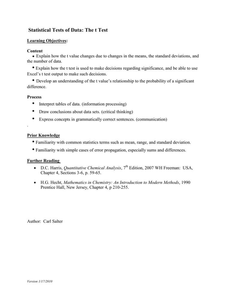
Statistical Tests of Data: The t Test
Learning Objectives:
Content
● Explain how the t value changes due to changes in the means, the standard deviations, and
the number of data.
• Explain how the t test is used to make decisions regarding significance, and be able to use
Excel’s t test output to make such decisions.
• Develop an understanding of the t value’s relationship to the probability of a significant
difference.
Process
•
•
•
Interpret tables of data. (information processing)
Draw conclusions about data sets. (critical thinking)
Express concepts in grammatically correct sentences. (communication)
.
Prior Knowledge
• Familiarity with common statistics terms such as mean, range, and standard deviation.
• Familiarity with simple cases of error propagation, especially sums and differences.
Further Reading

D.C. Harris, Quantitative Chemical Analysis, 7th Edition, 2007 WH Freeman: USA,
Chapter 4, Sections 3-6, p. 59-65.

H.G. Hecht, Mathematics in Chemistry: An Introduction to Modern Methods, 1990
Prentice Hall, New Jersey, Chapter 4, p 210-255.
Author: Carl Salter
Version 1/17/2010
Statistical Tests of Data: The t Test
Scientists often compare sets of similar measurements. For example, an analytical chemist might
compare two different methods for measuring the amount of carbon dioxide in air. Or a food
chemist might measure dissolved carbon dioxide in two different brands of soda.
Either way, we often must decide if the differences in the sets of measurements reflect
real differences between the two methods or the two samples, or if the differences are not likely
to be real and are probably the result of random error that is always present to some degree in any
measurement. Statisticians call this significance testing. The most important statistics about a
data set are its average (mean) and standard deviation; together they are called the summary
statistics of the set. (Admittedly there are other important statistics about a set of data—the
minimum and the maximum, for example—but it the average and the standard deviation that we
subject to significance testing.) Two sets of data could differ in their average values; they could
also differ in their standard deviation—either of these differences can be judged to be significant
and real or insignificant and probably the result of random error. While it is never possible to say
with absolute certainty whether or not a difference is real, it is possible to assign a probability.
We usually label an experimental difference “significant” when its probability of “realness” is
95% or better. Significant differences deserve an explanation; differences that are not significant
do not!
There are two tests designed to test summary statistics: the t test tests the difference of
two averages, and the F test tests the difference of two standard deviations. This activity will
examine the t test. Because there are three different variations of the t test, this activity is rather
long, and so it has been divided into two parts. Part 1 develops an understanding of how the t
test does its job, and Part 2 examines the three different types of t tests and how they can be
performed in Excel.
Part 1 Fundamental Concepts
Consider This
April and Betty each measure the absorbance of the same colored solution three times; each
student has her own absorption spectrometer. (Absorbance is unitless.)
Set 1
April
0.121
0.122
0.123
Betty
0.123
0.124
0.125
Consider possible claims regarding April and Betty’s data:
a. Betty’s absorption data are higher than April’s; therefore Betty’s spectrometer must somehow
be different from April’s, making it give higher measurements than April’s.
b. April’s absorption data are lower than Betty’s; therefore April must have somehow diluted
her sample slightly before she made her measurements.
c. Betty and April’s absorption data are a little different, but not by much, so maybe the
difference is entirely random.
Version 1/17/2010
Statistical Tests of Data
1
d. There’s no real difference between April’s and Betty’s data; the difference is within the limit
of performance of the two spectrometers.
1.
Which claim(s) say that the difference in April and Betty’s data is insignificant?
Which claim(s) says that the difference in their data is significant and “real”?
If two people claim that a difference is real, do they have to agree on the cause of the difference?
Explain.
2.
Are any of the claims clearly false given the available information? If your group has a
unanimous opinion, explain why you think so and write an explanation.
If one or more of your group believes a claim is true, would that person bet fifty dollars that the
claim is true? Would anyone in your group agree to take that bet?
The symbol Psignif represents the probability that the difference between April’s data and Betty’s
data is significant, that is, the difference is the result of some real difference in the sample or the
measuring routine. Pinsignif will represent the probability that the difference is insignificant; that
is, it is due to random error.
3.
Suppose that Psignif =0.85. What would be the value of Pinsignif? Explain.
What is the sum of Psignif and Pinsignif, and why?
Version 1/17/2010
Statistical Tests of Data
2
Consider the following possible sets of data that April and Betty might obtain. Set 1 is listed
again for easy comparison.
Set 1
April
0.121
0.122
0.123
Betty
0.123
0.124
0.125
Set 2
April
0.120
0.121
0.122
Set 3
Betty
0.124
0.125
0.126
April
0.121
0.122
0.123
Set 4
April
0.120
0.122
0.124
Betty
0.122
0.124
0.126
Set 5
April
0.122
0.122
0.122
Set 6
April
0.122
Betty
0.121
0.122
0.123
Betty
0.124
0.124
0.124
Set 7
Betty
0.124
April
0.121
0.121
0.122
0.122
0.123
0.123
Betty
0.123
0.123
0.124
0.124
0.125
0.125
4.
Consider set 2. Compared to set 1, which summary statistics—the average, the standard
deviation, or both--have changed?
Compared to set 1, what has happened to the value of Psignif? Explain your conclusion.
5.
Consider set 3. Compared to set 1, which summary statistics have changed?
Compared to set 1, what has happened to the value of Psignif? Explain your conclusion.
Version 1/17/2010
Statistical Tests of Data
3
6.
Based on your answers to the previous two questions, what should happen to Psignif as the
difference between the average values increases? Your answer should be a complete,
grammatically correct sentence.
7.
Consider set 4. Compared to set 1, which summary statistics have changed?
Compared to set 1, what has happened to the value of Psignif? Explain your conclusion.
8.
Consider set 5. Compared to set 1, which summary statistics have changed?
Compared to set 1, what has happened to the value of Psignif? Explain your conclusion.
9.
Based on your answers to the previous two questions, what should happen to Psignif as the
standard deviation of the measurements increases? Your answer should be a complete,
grammatically correct sentence.
10.
Suppose that April and Betty had made just one measurement on the sample, as in set 6.
Compared to set 1, what has happened to the value of Psignif? Explain your conclusion.
11.
Suppose that April and Betty each made six measurements, as in set 7. Compared to set
1, what has happened to the value of Psignif? Explain your conclusion.
12.
Based on your answers to the previous two questions, what should happen to Psignif as the
number of measurements increases? Your answer should be a complete, grammatically
correct sentence.
Version 1/17/2010
Statistical Tests of Data
4
13.
Discuss as a group: Based on the data in set 2, would you claim there is a significant
difference between April and Betty’s data? Would you bet fifty dollars on that claim?
14.
Based on the data in set 5, would you claim there is a significant difference between the
data? Would you bet fifty dollars on that claim?
15.
Develop a group summary of the effect that averages, standard deviations, and number of
data have on Psignif.
Version 1/17/2010
Statistical Tests of Data
5
Consider this
The difference between average values of two sets of measurements is a quantity derived from
the data, and as such it has an error. The error can be computed using the rules for the
propagation of error. Each step in the calculation requires a corresponding step of error
propagation.
Step 1: Computing the averages and their errors.
The standard deviation of an average value is s / n ; where s is the standard deviation of the
measurements and n is the number of measurements in the set. ( s / n is sometimes called the
standard error or the standard deviation in the mean. Throughout the remainder of this
activity, the former name will be used.) If we have two data sets, then we get the average x1 and
its error s x1 , and x 2 and its error s x2 , where
Standard error:
s xi 
si
ni
Step 2: Computing the difference and its error:
The error in the difference of two measurements is s12  s22 , the square root of the sum of the
squared errors. When we take the difference of two average values, x  x1  x 2 ,
and the Standard error of x is
s x1  x2  s x  s x21  s x22 .
The error in the difference of the averages is the square root of the sum of the squares of the
standard errors.
16.
Write the equation for sx using the original standard deviations of the measurements, s1
and s2. Simplify so that you use just one square root symbol.
s x =
17.
Examine the equation in Question 16. How will sx change if the standard deviations of
the measurements increase? How will sx change if the number of measurements increases?
18.
Relative error is the error in a quantity divided by the quantity itself. We’re interested in
the relative error of the differences in the averages—well, actually we’re interested in its
Version 1/17/2010
Statistical Tests of Data
6
reciprocal. Write a mathematical expression for the reciprocal of the relative error by
inserting the expression for sx into the following equation:
x

s x
Reciprocal of relative error:
19.
Develop a group summary: Does the mathematical expression in Questions 18 change as
you expect Psignif to change for different sets of data? Your summary should explain how the
quantity will change as the standard deviations of the measurements increases, how it will change
as the number of measurements increases, how will it will change as the difference of the average
values increase.
Consider this
The quantity in Question 18 is what analytical chemists generally call the t value; t is defined as
the absolute value of the difference of the means divided by the error in the difference. A t value
is simply the unsigned difference divided by its error. A t value is also the reciprocal of
relative error.
20.
Write expressions for the t value, first using the standard errors, and then using the
standard deviations in the measurements.
t
x
s x

x1  x 2

x1  x 2
Why do we use the absolute value? Why can we disregard the sign of the difference?
Version 1/17/2010
Statistical Tests of Data
7
21.
As a group, verify that for every set of April and Betty’s data, n1 = n2 and s1 = s2. Write
an equation for t given these special conditions. Since they are equal, use s and n without
subscripts in this special formula.
22.
Using the formula you derived in Question 21, fill in the following table for each set of
data. Divide up the work among the members of your group.
Set
1
x1  x 2
0.002
s
n
0.001
t
3
2.449
Unknown
1
NA
0.0009
6
3.873
2
3
4
0.002
5
6
7
0.002
There are two cases where it is not possible to compute t. What problems prevent you from
computing t?
23.
Discuss as a group: Does t change as you expected Psignif to change in these data sets? Do
t and Psignif have the same trend as the data changes? Give two examples supporting your answer
and explain your reasoning.
24.
Discuss as a group: What is the range of possible numeric values for t? (That is, what
values could it take on?)
Version 1/17/2010
Statistical Tests of Data
8
What is the range of possible numeric values for Psignif?
Could t be the same numerical quantity as Psignif? Explain why or why not.
Version 1/17/2010
Statistical Tests of Data
9
Consider this
It is possible to use the t value to determine Psignif -- but right now all we need to do is find out if
Psignif ≥ 0.95. There is a table of t values that tells us when t is big enough to know that Psignif ≥
0.95. The table is given below. It is a portion of the Student’s t table for two-tailed
distributions. (Excel’s TINV function will provide these values.)
Degrees of tcritical for
freedom
Psig ≥0.95
1
12.706
2
4.303
3
3.182
4
2.776
5
2.571
6
2.447
7
2.365
8
2.306
9
2.262
10
2.228
15
2.131
20
2.086
25
2.060
30
2.042
40
2.021
50
2.009
60
2.000
120
1.980
∞
1.960
When you compare a t value for experimental data against a tcritical value, you are doing a t
test. In different books the t value computed from the data may be called tcalculated or tcalc or tdata or
tstat or simply t; the t value from the Student’s t table is usually called tcritcal or ttable. There are
several types of t tests, but in all cases when tcalculated > tcritical, the difference being tested is
considered significant.
For the rest of Part 1 of this activity, and also in Part 2, we will use the symbols tcalc and
tcrit. tcalc is computed from the data; tcrit comes from the table. When the tcalc > tcrit, we know
that Psignif >0.95, and we can conclude that the difference in the means is real and significant.
25.
What would we conclude about Psignif if tcalc equaled tcrit?
26.
To find a particular tcrit value in the Student’s t table, what quantity do you need?
Version 1/17/2010
Statistical Tests of Data
10
The number of degrees of freedom is the total number of data minus the number of averages that
were computed from the data.
ndf  n  p
Degrees of freedom:
where p is the number of averages that were computed.
27.
If April and Betty have each collected 3 data, and they each compute 1 average value
from their data, they each have 2 degrees of freedom.
What is the total degrees of freedom from both sets of data?
How many degrees of freedom are there when April and Betty each collect 6 data?
28.
Complete the following table for each set of data. Enter t from your previous table as
tcalc. Divide the work among the members of your group.
Set
1
n
tcalc
3
ndf
tcrit
Significant
?
no
2.228
YES!
2.449
2
4
3
4
5
6
1
NA
7
6
3.873
0
29.
Discuss in your group: Among the five cases where it was possible to compare tcalc and
tcrit, which ones showed a significant difference? Are there any cases where you and your group
are surprised that the Psignif is greater than 0.95?
30.
Which set appears to have the most significant difference? What makes you think that it
is most significant?
What is it about this data set that leads to this result?
Would you or anyone in your group bet fifty dollars that this difference is significant?
Version 1/17/2010
Statistical Tests of Data
11
31.
What question does the t test answer?
32.
For group discussion: How confident are you that you understand how the t test is used?
33.
As a group, describe your ability to read statistical tables.
Version 1/17/2010
Statistical Tests of Data
12
Applications
34.
Consider the two cases where a t test could not be completed. How are the two cases
different? Based on the behavior of tcrit in the Student’s t table, what conclusions can you draw
about the significance of the differences in these two cases.
35.
Consider set 1. Generate a set of three data that is significantly different from April’s
data but not significantly different from Betty’s data.
36.
Suppose you had two data sets each containing four data, and the two sets have equal
standard errors. How far apart would the two means have to be, in terms of the standard error,
for the t test to yield a significant difference?
37.
Blood is drawn from a patient suffering from hypoparathyroidism to determine her serum
calcium concentration. Five replicate analyses yield a mean of 8.11 mg/dL with a standard error
of 0.16 mg/dL. Two weeks later after drug therapy her serum calcium is measured again; now
five measurements yield 8.40 mg/dL with a standard error of 0.19 mg/dL. Has the patient’s
serum calcium changed?
38.
Sally measures the amount of CO2 in a pint soda bottle by weight loss; she shakes the
bottle vigorously and then slowly opens the cap, letting the gas escape. Three measurements on
Brand X indicate a loss of 2.2 ± 0.2 g of gas, while three measurements on Brand Y shows a loss
2.4 ± 0.3 g. (The ± indicates standard error.) Do Brands X and Y have different amount of CO2?
39.
Suppose that Bob and Bill make repeated measurements of the amount of iron in two iron
ore samples. Bob gets 20.14%, 20.14%, 20.20%, and 20.26% Fe for his ore sample, and Bill gets
20.02%, 20.08%, 20.11% , and 20.18% Fe for his sample. Do the two samples have different
iron percentages?
Version 1/17/2010
Statistical Tests of Data
13
Part 2 Excel Implementation and Variations
The t test that we have been considering is called a Comparison of Two Means, or a
Comparison of Replicate Measurements. This test tells us if x , the difference in the average
value of two sets of measurements, is statistically significant.
Review: In Part 1 we learned that the value tcalc is the ratio of the difference of the means to the
standard error in that difference.
x
t calc 
s x
As tcalc increases, the probability of a significant difference increases.
We saw that tcalc increases with increasing difference in the means, increasing numbers of data,
and decreasing standard deviations. To do a t test, tcalc is compared with tcrit, a value that is
selected from the Student’s t table based on the number of degrees of freedom ndf. If tcalc > tcrit,
then the probability of a significant difference, Psignif , is greater than 0.95 and the difference is
considered significant.
Consider this
In the examples we examined in Part 1, April and Betty always had the same number of data, and
the standard deviations of their measurements were always equal. Clearly this will not always be
the case. In set 2 below April and Betty have different numbers of data and different standard
deviations. The mean and variance are listed for each group of data. (The variance ν is the
square of the standard deviation.)
April
0.121
0.122
0.123
x
ν
0.122
Set 1
Betty
0.123
0.124
0.125
10x10-07
0124
10x10-07
Set 2
April Betty
0.121 0.123
0.122 0.123
0.123 0.124
0.124
0.125
0.125
0.122 0.124
10x10-07 8x10-07
Set 3
April
Betty
0.121
0.123
0.121
0.123
0.122
0.124
0.122
0.124
0.123
0.125
0.123
0.125
0.122
0.124
8x10-07
8x10-07
1.
Consider tcalc for each of these data sets. Rank the sets in the order that you expect tcalc to
fall, from lowest to highest, and explain your prediction.
2.
Test your predicted order. For each set of data, compute tcalc.
Version 1/17/2010
Statistical Tests of Data
14
t calc 
Comparison of Two Means
x
s x

x1  x2
s12 s 22

n1 n2
Divide the work among your group.
Was your predicted order correct?
3.
Determine tcrit for set 2. Is the difference between April’s and Betty’s means significant
in this case?
Here are the results of a t test performed on Set 2 in Excel using the t-test: Two-Sample
Assuming Equal Variances tool in the Data Analysis Toolpak. The default values of the test were
used.
Mean
Variance
Observations
Pooled Variance
Hypothesized
Mean Difference
Df
t Stat
P(T<=t) one-tail
t Critical one-tail
P(T<=t) two-tail
t Critical two-tail
April
0.122
0.000001
3
8.57E-07
Betty
0.124
8E-07
6
0
7
-3.05505
0.009226
1.894579
0.018452
2.364624
*This Excel test reports a negative value of t. In Excel input window, if the columns containing April and
Betty’s data are swapped, the t test tool will report a t Stat equal to +3.055. For this type of t test, ignore a
negative sign in a t value from Excel!
4.
As a group, examine the t test results from Excel. Based solely on the Excel results, is
the difference between April’s and Betty’s means significant? Which values in the output did
you use to make your decision?
Version 1/17/2010
Statistical Tests of Data
15
Here are the essential test results from Excel for all three sets.
Pooled Variance
df
t Stat
P(T<=t) two-tail
t Critical two-tail
Set 1
0.000001
4
2.44949
0.070484
2.776445
Set 2
8.57E-07
7
3.05505
0.018452
2.364624
Set 3
8E-07
10
3.87298
0.003094
2.228139
5.
Compare the results from Excel with your results in Questions 2 and 3. Check tcalc, ndf,
and tcrit. Can you assign these values to the Excel output? Are there any values that disagree with
your results?
You should find that your value of tcalc for set 2 is slightly less than the “t Stat” value from Excel
(though it doesn’t affect the decision that the means are significantly different.) However, your
tcalc for sets 1 and 3 agree with Excel!
6.
Compare the quantities labeled Pooled Variance with the variances listed for each group of
data. What conclusion can you draw about the value of the pooled variance when the individual
variances are equal?
The pooled standard deviation is a way to combine standard deviations for two sets of
measurements if the variances are essentially equal. It simplifies the formula for the standard
error of the difference.
s pooled 
(n1  1) s12  (n2  1) s 22
n1  n2  2
The pooled variance is  pooled  s 2pooled
Using the pooled standard deviation, we can express s x more simply:
s x  s pooled
1
1

n1 n2
Version 1/17/2010
Statistical Tests of Data
16
8.
Show that, using the pooled standard deviation, the formula for tcalc becomes
x1  x2
n1 n2
when the variances are roughly equal.
t calc 
s pooled n1  n2
9.
The t test used in Excel made the assumption that the variances of the two sets of data
were equal. Are the two variances in Set 2 equal?
In another activity we will introduce a test called the F test that will determine if the variances are
significantly different. There are actually two forms of the t test, and the choice of t test is based
on the result of the F test. If the variances are not significantly different, then t is computed using
the formula in Question 8 using spooled. If the variances are significantly different, then spooled is
not used, and tcalc is computed using the formula in Question 2. But there are other differences as
well; these will be covered in the F test activity.
In theory, we should always do an F test before we do the t test--but in practice the F test
is often skipped. In routine chemical analysis on small data sets that come from the same
measuring device, it is reasonable to assume that the variances are not significantly different,
even if they are not exactly equal. But it is always safer to test that assumption than to proceed in
error!
10.
In the Excel output, there is a quantity labeled P(T<=t) two-tail. This quantity is a
probability. Is it Psignif or Pinsignif? Explain your choice.
* One of the default values for the t test is “alpha=0.05”.
“Alpha” is Pinsignif; alpha = 0.05 makes the t test use a tcrit consistent with a 95% probability of a
real difference. Statisticians usually based their tables on Pinsignif, so be careful when you are
looking at P values--If you see an α, assume the α probabilities are Pinsignif.
11.
For group discussion: If you had to bet fifty dollars on something, what would be the
better bet: that the difference in set 2 is real, or that you will draw one card from a standard pack
of 52 cards and not draw a deuce? Explain.
Version 1/17/2010
Statistical Tests of Data
17
12.
As a group, write a set of instructions that would let a lab technician read the output of an
Excel t test and come to a conclusion about significance.
Consider this
The most common type of t test is the Comparison of Means, but there are two other important
applications of the t test. Both can be considered special cases of the Comparison of Means.
The first is the Comparison Against an Accepted Value. Often we want to compare
one set of measurements against a value that is “known” or accepted as “true”. The true value is
widely regarded as “above reproach” and can be assumed to have no error.
13.
For group discussion: If the accepted value has no error, what is its “standard deviation”?
14.
Assuming that x 2 = True and sT rue = 0, show that the formula for tcalc for the Comparison
Against an Accepted Value becomes
x1  True
x1  True
t calc 

n1 or simply
s x1
s1
Comparison Against Accepted Value t calc 
x  True
s
n
15.
April and Betty are told that the accepted value for the absorption of their solution is
0.122. Using the data in set 2, determine whether April and Betty’s average values are
significantly different from 0.122.
Version 1/17/2010
Statistical Tests of Data
18
Consider this
Another type of t test is the Comparison of Paired Values or Comparison of Individual
Differences. It is used to test the significance of a series of differences that result from paired
measurements on the same sample.
Suppose that April and Betty get six different colored solutions and measure the
absorptions of the solutions using their instruments. They now have six pairs of measurements,
and they can compute six differences, one difference for each pair: d1=ABetty1-AApril1, d2=AB2AA2, d3, d4, d5, and d6. From these values of d they compute the average difference d , and sd,
the standard deviation of the differences.
16.
For group discussion: April and Betty hope that their measurements agree. What values
would they like to get for d and sd?
17.
Realistically, since there is always some random error present in any measurement, April
and Betty will not get sd=0. If their measurements mostly agree, should d >sd or should
d <sd? Explain your group’s reasoning.
18.
April and Betty need to test d to see if it is significantly different than 0. (Even though
they’re hoping that it won’t be!) Show that if x = d and True=0, the formula for tcalc for the
Comparison of Paired Values becomes
t calc 
d
sd
or simply
Comparison of Paired Values
t calc 
d
sd
n
19.
Since April and Betty are testing an average based on six values (even though there were
originally twelve measurements), for their paired t test, n=6. So what is ndf?
Version 1/17/2010
Statistical Tests of Data
19
20.
Assume that April and Betty get identical measurements for three solutions and get a
difference of +0.001 for the other three. (Betty’s values are always higher.)
Generate a set of data consistent with the assumption.
Obviously d =+0.0005. Find sd. Is it > or < d ?
Compute tcalc.
Find tcrit. Are April and Betty getting significantly different measurements? Explain your
conclusion in a complete sentence.
21.
Most Student’s t tables have columns of tcrit values for other values of Psignif. Usually
these probabilities are called “confidence levels” and are given in percentages. For example, for
5 degrees of freedom, you would find the following values:
ndf
50%
90%
95%
98%
99%
99.5%
99.9%
5
0.727
2.015
2.571
3.365
4.032
4.773
6.869
Based on the tcrit values for ndf=5 and the tcalc you computed in Question 20, bracket the value of
Psignif:
_________< Psignif < _________
Version 1/17/2010
Statistical Tests of Data
20
22.
Here is the output from Excel’s Data Analysis ToolPak for a t test: Paired Two Sample
for Means. The input data was consistent with Question 20.
Mean
Variance
Observations
Pearson Correlation
Hypothesized Mean
Difference
df
t Stat
P(T<=t) one-tail
t Critical one-tail
P(T<=t) two-tail
t Critical two-tail
April
0.158
0.017432
6
0.999992
Betty
0.1585
0.01745
6
0
5
-2.23607
0.037793
2.015049
0.075587
2.570578
Since April’s data are always less than or equal to Betty’s and April’s data were placed in the
first column, the value of t Stat is negative. Otherwise, is it consistent with your value of tcalc?
Explain.
What other values do you recognize in the Excel output? Do they match your values?
23.
Excel reports that P(T<=t) two-tail is 0.076. What does this indicate about Psignif and
Pinsignif? Is it consistent with your conclusion about Psignif in Question 21?
24.
As a group, review your set of instructions for a lab technician in Question 12. Would
they work for the Paired Two-Sample t test? If not, modify them accordingly and write them
below.
25.
What are the three types of t tests, and what questions do they answer?
Version 1/17/2010
Statistical Tests of Data
21
26.
For group discussion: How confident are you that you will know which t test to use in a
given situation?
27.
As a group, describe your ability to read Excel output.
Version 1/17/2010
Statistical Tests of Data
22
Applications
28.
Insert the data from Set 2 into Excel and verify that you get the Excel output shown in
Question 3.
29.
Suppose you had a set of four data with a certain mean and standard error. Suppose there
is an accepted value for these data. In terms of the standard error, how far away from the
accepted value would the mean have to be for the t test to determine a significant difference?
30.
Suppose that Bob and Bill make repeated measurements of the amount of iron in two iron
ore samples. Bob gets 20.14%, 20.14%, 20.20%, and 20.26% Fe for his ore sample, and Bill gets
20.02%, 20.08%, 20.11% , and 20.18% Fe for his sample. Bob and Bill learn that their samples
are from the same source, and that the accepted value is 20.09% Fe. Are Bob’s and Bill’s means
significantly different from the accepted value?
31.
Suppose you have a set of seven paired samples with an average difference of d and a
standard error in the difference of s d  . In terms of the standard error, how big must d be for the
paired t test to determine a significant difference?
32.
Insert the data you generated in Question 20 into Excel, perform the Paired Two-Sample t
test, and show that you get the results displayed in Question 22.
33.
Eight patients are treated for hypoparathyroidism using a drug therapy. Before the
treatment, the eight patients have serum calcium levels of 8.12, 7.98, 8.06, 7.65, 8.20, 8.08, 8.15,
and 8.22 mg/dL. After treatment, the serum levels were 8.22, 8.02, 8.08, 7.96, 8.31, 8.28, 8.20,
and 8.33 mg/dL. Was there a significant increase in serum calcium after the patients were given
the treatment? Which t test should be used to answer this question?
Version 1/17/2010
Statistical Tests of Data
23