Methodologies for Population/Quantitative Genetics
Animal Science 562
Matrix Algebra
Vectors and Matrices: Basic Concepts
We begin by introducing some very basic concepts that are essential for algebraic
explanations of subsequent statistical techniques. The intent is to provide a brief refresher of the
concepts which will be used throughout the semester for those who have not been previously
exposed to the rudiments of matrix algebra. Toward the end, derivations are presented for
particular algebraic forms that repeatedly appear in papers dealing with mixed models.
VECTORS
Many concepts, such as observed measurements of a trait, factors of a model, or an
animal's breeding value cannot be adequately quantified as a single number. Rather, several
different measurements y1, y2,...ym are required.
Definition 1) An m-tuple of real numbers (y1, y2,...ym) arranged in a column is called a vector
and is denoted by a boldfaced, lowercase letter. Other references might use an ~ underline in
place of a boldface letter.
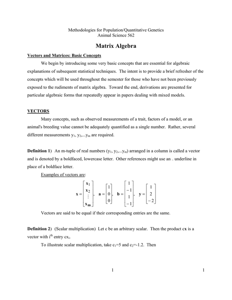
Examples of vectors are:
⎡1⎤
⎡ x1 ⎤
⎡
⎤
1
⎢− 1⎥
⎢x ⎥
⎢ ⎥
2⎥
⎢
x=
, a = ⎢0⎥, b = ⎢ ⎥, y =
⎢1⎥
⎢ M ⎥
⎢⎣0⎥⎦
⎢ ⎥
⎢ ⎥
⎣− 1⎦
⎣x m ⎦
⎡ 1⎤
⎢ ⎥
⎢2 ⎥
⎢⎣− 2⎥⎦
Vectors are said to be equal if their corresponding entries are the same.
Definition 2) (Scalar multiplication) Let c be an arbitrary scalar. Then the product cx is a
vector with ith entry cxi.
To illustrate scalar multiplication, take c1=5 and c2=-1.2. Then
1
1
Animal Science 562
Matrix Algebra
⎡ 1 ⎤ ⎡5⎤
⎡ 1⎤
⎢ ⎥ ⎢ ⎥
⎢ ⎥
. *⎢ 2 ⎥=
c1y = 5 * ⎢ 2 ⎥ = ⎢10⎥ , and c 2 y = − 12
⎢⎣− 2⎥⎦ ⎢⎣10⎥⎦
⎢⎣− 2⎥⎦
⎡ − 12
. ⎤
⎢
⎥
⎢− 2.4⎥
⎢⎣ 2.4 ⎥⎦
Definition 3) (Vector addition) The sum of two vectors x and y, each having the same number
of entries, is that vector
z = x + y, with ith entry zi = xi + yi
⎡3⎤ ⎡ 1 ⎤
⎢ ⎥ ⎢ ⎥
⎢− 1⎥ + ⎢ 2 ⎥ =
⎢⎣ 4 ⎥⎦ ⎢⎣− 2⎥⎦
x + y =
Thus,
⎡ 4⎤
⎢ ⎥
⎢ 1⎥
⎢⎣ 2⎥⎦
z
Definition 4) The vector y = a1x1 + a2x2 + ... + akxk is a linear combination of the vectors x1,
x2,...xk.
Definition 5) A set of vectors x1, x2, ... xk is said to be linearly dependent if there exist k
numbers (a1, a2, ... , ak), not all zero, such that
a1x1 + a2x2 + ... + akxk = 0.
Otherwise the set of vectors is said to be linearly independent.
If one vector, for example x1, is 0, the set is linearly dependent (let ai be the only nonzero
coefficient from Definition 5).
The familiar vectors with a one as an entry and zeros elsewhere are linearly independent.
For m=4,
⎡1⎤
⎡ 0⎤
⎢ 0⎥
⎢1⎥
⎢
⎥
x1 =
, x 2 = ⎢ ⎥, x 3 =
⎢ 0⎥
⎢ 0⎥
⎢ ⎥
⎢ ⎥
⎣ 0⎦
⎣ 0⎦
so
2
⎡ 0⎤
⎡ 0⎤
⎢ 0⎥
⎢ 0⎥
⎢ ⎥, x = ⎢ ⎥
4 ⎢ 0⎥
⎢1⎥
⎢ ⎥
⎢ ⎥
⎣ 0⎦
⎣1⎦
Animal Science 562
Matrix Algebra
⎡a11 + a 2 0 + a 3 0 + a 4 0⎤
⎢a 0 + a 1 + a 0 + a 0⎥
1
2
3
4 ⎥
=
0 = a1x1 + a 2 x 2 + a 3x 3 + a 4 x 4 = ⎢
⎢a1 0 + a 2 0 + a 31 + a 4 0⎥
⎢
⎥
⎣a1 0 + a 2 0 + a 3 0 + a 4 1⎦
⎡ a1 ⎤
⎢a ⎥
⎢ 2⎥
⎢a 3 ⎥
⎢ ⎥
⎣a 4 ⎦
implies a1 = a2 = a3 = a4 = 0.
As another example, let k=3 and m=3.
⎡1⎤
⎡2⎤
⎡0⎤
⎢⎥
⎢ ⎥
⎢ ⎥
x1 = ⎢1⎥ , x 2 = ⎢ 5 ⎥ , x 3 = ⎢ 1 ⎥
⎢⎣1⎥⎦
⎢⎣− 1⎥⎦
⎢⎣− 1⎥⎦
Then
2x1 - x2 + 3x3 = 0.
Thus x1, x2, x3 are a linearly dependent set of vectors since any one of them can be
written as a linear combination of the others (for example, x2 = 2x1 + 3x3).
Definition 6) The inner (or dot) product of two vectors x and y with the same number of entries
is defined as the sum of component products
x1y1 +x2y2 + ... + xmym.
We use the notation x'y or y'x to denote this inner product.
MATRICES
Definition 7) A mxk matrix, generally denoted by boldface uppercase letters like A, R, and so
forth, is a rectangular array of elements having m rows and k columns. As was the case for
vectors an ~ underline can be used in place of boldface letters (e.g. ).
Definition 8) The dimension of an mxk matrix is the ordered pair (m,k); m is the row dimension
and k is the column dimension.
An mxk matrix, call it A, of arbitrary constants can be written
3
Animal Science 562
Matrix Algebra
⎡ a11 a12
⎢a
21 a 22
A mxk = ⎢
⎢ M
M
⎢
⎣a m1 a m 2
L a1k ⎤
L a 2k ⎥
⎥
O
M ⎥
⎥
L a mk ⎦
or more compactly as AmXk={aij}, where the index i refers to the row and the index j refers to the
column.
Definition 9) (Scalar multiplication). Let c be an arbitrary scalar and A={aij}. Then
cAmXk=AmXkc=BmXk={bij}, where bij=caij=aijc, i=1,2,...,m, and j=1,2,...,k.
Multiplication of a matrix by a scalar produces a new matrix whose elements are the
elements of the original matrix, each multiplied by the scalar.
Definition 10) (Matrix multiplication). The product AB of an mxn matrix A={aij} and an nxk
matrix B={bij} is the mxk matrix C whose elements cij are given by
n
c ij = ∑ a iι bιj
ι=1
Note that for the product AB to be defined, the column dimension of A must equal the row
dimension of B. Then the row dimension of AB equals the row dimension of A and the column
dimension of AB equals the column dimension of B.
Result 10a)
For all matrices A, B, and C ( dimensions such that the indicated products
are defined) and a scalar c,
a)
c(AB) = (cA)B
b)
A(BC) = (AB)C
c)
A(B+C) = AB + AC
d)
(B+C)A = BA + CA
e)
(AB)' = B'A'
There are several important differences between the algebra of matrices and the algebra
of real numbers. Two of these differences are:
4
Animal Science 562
Matrix Algebra
a)
Matrix multiplication is, in general, not commutative. That is, in general
AB ≠ BA.
b)
Let 0 denote the zero matrix, that is, the matrix with zero for every
element. In the algebra of real numbers, if the product of two numbers,
ab, is zero, then a=0 or b=0. In matrix algebra, however, the product of
two nonzero matrices may be a zero matrix. Hence,
(AmXn)(BnXk) = 0
does not imply that A=0 or B=0.
Definition 11) Inverse of Partitioned Matrices (Searle, 1966 p.210). Obtaining the inverse of a
matrix can often be simplified by partitioning it into four sub-matrices in a manner such that
those at the top left and bottom right are square; i.e.,
M =
⎡A B ⎤
⎢C D ⎥
⎣
⎦
where A and D are square. If the corresponding partitioned form of M-1 is
⎡X Y ⎤
M −1 = ⎢
⎥
⎣Z W⎦
Then
Z = -D-1CX
X = (A-BD-1C)-1
Y = -A-1BW
W = (D-CA-1B)-1
The procedures simplify when M is symmetric, M=M', for then A=A', C=B', D=D', and X=X',
Z=Y', and W=W'. That is,
⎡ A B⎤
−1
M=⎢
⎥ and M =
'
B
D
⎣
⎦
⎡X Y ⎤
⎢Y ' W ⎥
⎣
⎦
One will encounter alternate expressions depending on the existence of A-1 or D-1 and the
ease of computation.
Procedure a (Requires the existence of D-1 but not A-1).
X = (A-BD-1B')-1
Y = -XBD-1
5
Animal Science 562
Matrix Algebra
W = D-1-Y'BD-1
Procedure b (Requires the existence of A-1 but not D-1).
W = (D-B'A-1B)-1
Y = -A-1BW
X = A-1-YB'A-1
Definition 12) Direct Sum (Searle, 1982 p. 283). Direct sums and direct products are matrix
operations defined in terms of partitioned matrices. The direct sum of two matrices A and B is
defined as
A⊕B =
⎡A 0 ⎤
⎢ 0 B⎥
⎣
⎦
and extends very simply to more than two matrices
⎡A 0 0 ⎤
⎥
⎢
A ⊕ B ⊕ C = ⎢0 B 0⎥
⎢⎣ 0 0 C⎥⎦
The definition and its extensions apply whether or not the submatrices are of the same order; and
all null matrices are of appropriate order. For example,
⎡1 2 3 0 0⎤
⎡ 6 7⎤
⎥
⎢
1 2 3 ⊕⎢
= ⎢ 0 0 0 6 7⎥
⎥
⎣8 9⎦
⎢⎣ 0 0 0 8 9⎥⎦
[
]
transposing a direct sum gives the direct sum of the transposes.
Definition 13) Direct Product (Searle, 1982 p. 265). The direct product of two matrices ApXq and
BmXn is defined as
A pxq ⊗ Bmxn
⎡a B L a B ⎤
1q
⎥
⎢ 11
O
M ⎥
= ⎢ M
⎢a B L a B⎥
pq ⎦
⎣ p1
6
Animal Science 562
Matrix Algebra
A direct product matrix is partitioned into as many submatrices as there are elements of A, each
submatrix being B multiplied by an element of A. It has order mpxqn. For example,
[1
⎡ 6 7 12 14 18 21⎤
⎢8 9 16 18 24 27⎥
⎣
⎦
⎡ 6 7⎤
2 3 ⊗⎢
⎥ =
⎣8 9⎦
]
Direct products have many useful and interesting properties:
a) In contrast to (AB)'=B'A', we have (A⊗B)'=A'⊗B'
b) For vectors x and y, x'⊗y = yx' = y⊗x'
c) For a scalar l, l⊗A = lA = A⊗l = Al
d) For partitioned matrices, although
[ A1
[
]
A2 ⊗ B
A ⊗ B1 B2
]
=
≠
[ A1 ⊗ B
[ A ⊗ B1
]
A ⊗ B2 ]
A2 ⊗ B
Definition 14) Differentiation.
∂w / ∂x = A' = A if A is symmetric.
a) w = Ax
∂w / ∂x = Ax + A'x = 2Ax if A is symmetric.
b) w = x'Ax
s
c) V = ∑ Vi σ i2
∂V / ∂σk2 = Vk for k ≤ s and k ≥ 1.
i=1
s
d) w = log |V|, V = ∑ Viσ i2
∂w / ∂σk2 = tr (V-1 ∂V/∂σk2) = tr (V-1Vk).
i=1
Definition 15) Inverse of V.
then V-1 = R-1-R-1Z(Z'R-1Z + G-1)-1Z'R-1
a) V = ZGZ' + R
Proof: Show that VV-1 = I
b) Z'V-1 = G-1(Z'R-1Z + G-1)-1Z'R-1
c) The above equalities are used many times in variance component estimation methods.
Try to memorize these results.
7
Animal Science 562
Matrix Algebra
There are a number of ways to find the inverse of a matrix. Two common approaches
are:
a) Row-wise reduction
b) Determinants
1. Find the determinant of a matrix.
2. Divide the determinant into the determinant of each principal cofactor matrix.
The cofactor matrix is the matrix remaining after deleting all row and column
elements with the same subscripts for the element you seek.
3. If the sum of the row and column subscript is an odd number, multiply the
coefficient by minus one.
4. Repeat b and c for all elements and take the transpose of the matrix.
Whichever method is best depends on the elements in the original matrix. I have found the
methods of determinants works well for 2x2 and 3x3 matrixes, but I do not recommend it for
larger matrices.
A 2x 2
Example 1.
⎡1 2⎤
= ⎢
⎥
⎣ 3 4⎦
The determinant, D, is D = 1*4 - 3*2 = -2.
A
−1
1
= −
2
⎡− 2 1 ⎤
⎡ 4 − 2⎤
⎢− 3 1 ⎥ = ⎢ 1 1 − 1 ⎥
⎢⎣ 2
⎣
⎦
2 ⎥⎦
Check that AA-1=I. The determinant is negative and diagonal elements of the inverse are
negative. This is not a general result, a least-squares coefficient matrix will have a positive
determinant and all diagonal elements of the inverse are positive.
8
Animal Science 562
Matrix Algebra
⎡ 1 2 3⎤
⎥
⎢
Example 2. A 3x3 = ⎢ 4 5 6⎥ →
⎢⎣ 7 8 9⎥⎦
c1
c2
c3
1
2
3
1
2
4
5
6
4
5
7
8
9
7
8
d1
d2
d3
The determinant, D = c1 + c2 + c3 - d1 - d2 - d3 where
c1 = a11 * a22 * a33
d1 = a31 * a22 * a13
c2 = a12 * a23 * a31
d2= a32 * a23 * a11
c3 = a13 * a21 * a32
d3= a33 * a21 * a12
as defined by the arrows. D=0, therefore there is a linear dependency among columns of the
matrix (i.e. 2x2-x1=x3, where x1, x2, and x3 are columns of the matrix A).
⎡1 2 5⎤
⎥
⎢
A 3x3 = ⎢ 6 7 9 ⎥
⎢⎣10 11 13⎥⎦
Example 3.
The determinant, D, is 1*7*13 + 2*9*10 + 5*6*11 - 10*7*5 - 11*9*1 - 13*6*2 = 91 + 180 +
330 - 350 - 99 - 156 = -4.
⎡ − 8 12 − 4⎤
1
⎥
⎢
A −1 = − ⎢ 29 − 37 9 ⎥
4
⎢⎣− 17 21 − 5⎥⎦
′
⎡2
⎡ − 8 29 − 17⎤
− 7.5
4.25 ⎤
1⎢
⎥
⎢
⎥
= − ⎢ 12 − 37 21 ⎥ = ⎢− 3 9.25 − 5.25⎥
4
⎢⎣ 1 − 2.25 125
⎢⎣− 4
− 5 ⎥⎦
9
. ⎥⎦
References
Mrode, R.A., 1996. Linear Models for the Prediction of Animal Breeding Values. CAB
International. Wallingford,U.K.
Searle, S.R. 1966. Matrix Algebra for the Biological Sciences : Including Applications in
Statistics. John Wiley & Sons, Inc., New York, NY.
Searle, S.R. 1982. Matrix Algebra Useful for Statistics. John Wiley & Sons. New York, NY.
9
Animal Science 562
Matrix Algebra
Harville, D. A. 1997. Matrix Algebra from a Statistician’s Perspective. Springer. New York, NY.
Ciarlet, P. G. 1988. Introduction to numerical linear algebra and optimisation. Cambridge
University Press, New York.
Purpose: to give a thorough description, and a rigorous mathematical analysis, of some of
the most commonly used methods in Numerical Linear Algebra and Optimisation.
Datta, B. N. 1994. Numerical Linear Algebra and Applications. Brooks/Cole Publishing
Company, New York.
Purpose: can be used in both undergraduate and beginning graduate courses, as well as
by working scientists and engineers for self study and reference. Special features:
applications- computational problems accompanied by real-life examples; recent
research- ; explanation of concepts; fundamental linear algebra problems;
examples with MATLAB.
Hill, D. R. 1987. Experiments in Computational Matrix Algebra. Random House, New York.
Purpose: programming with MATLAB.
10