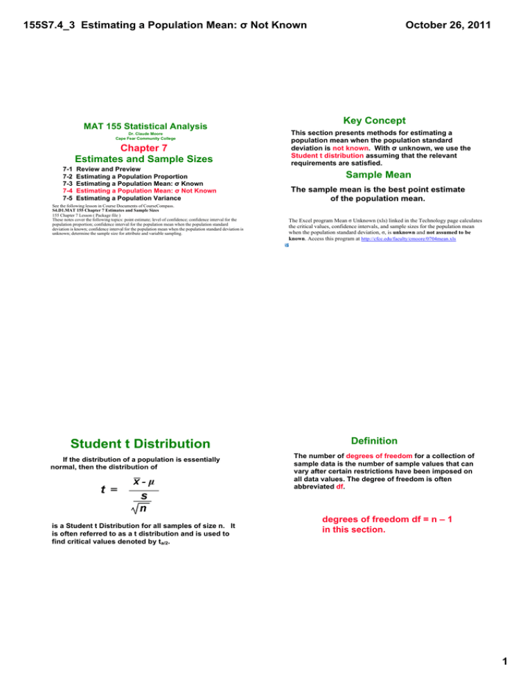
155S7.4_3 Estimating a Population Mean: σ Not Known
MAT 155 Statistical Analysis
Dr. Claude Moore
Cape Fear Community College
Chapter 7
Estimates and Sample Sizes
7­1 Review and Preview
7­2 Estimating a Population Proportion
7­3 Estimating a Population Mean: σ Known
7­4 Estimating a Population Mean: σ Not Known
7­5 Estimating a Population Variance
See the following lesson in Course Documents of CourseCompass.
S4.D1.MAT 155 Chapter 7 Estimates and Sample Sizes
155 Chapter 7 Lesson ( Package file )
These notes cover the following topics: point estimate; level of confidence; confidence interval for the population proportion; confidence interval for the population mean when the population standard deviation is known; confidence interval for the population mean when the population standard deviation is unknown; determine the sample size for attribute and variable sampling.
Student t Distribution
If the distribution of a population is essentially normal, then the distribution of
is a Student t Distribution for all samples of size n. It is often referred to as a t distribution and is used to find critical values denoted by ta/2.
October 26, 2011
Key Concept
This section presents methods for estimating a population mean when the population standard deviation is not known. With σ unknown, we use the Student t distribution assuming that the relevant requirements are satisfied.
Sample Mean
The sample mean is the best point estimate of the population mean.
The Excel program Mean σ Unknown (xls) linked in the Technology page calculates the critical values, confidence intervals, and sample sizes for the population mean when the population standard deviation, σ, is unknown and not assumed to be known. Access this program at http://cfcc.edu/faculty/cmoore/0704mean.xls
Definition
The number of degrees of freedom for a collection of sample data is the number of sample values that can vary after certain restrictions have been imposed on all data values. The degree of freedom is often abbreviated df.
degrees of freedom df = n – 1
in this section.
1
155S7.4_3 Estimating a Population Mean: σ Not Known
Margin of Error E for Estimate of μ (With σ Not Known)
October 26, 2011
Notation
µ = population mean
= sample mean
s = sample standard deviation
n = number of sample values
E = margin of error
tα/2 = critical t value separating an area of α/2 in the right tail of the t distribution
Table A­3 lists values for tα/2 Confidence Interval for the Estimate of μ (With σ Not Known)
Procedure for Constructing a Confidence interval for µ
(With σ Unknown)
tα/2 found in Table A­3
2
155S7.4_3 Estimating a Population Mean: σ Not Known
October 26, 2011
Example:
Example:
A common claim is that garlic lowers cholesterol levels. In a test of the effectiveness of garlic, 49 subjects were treated with doses of raw garlic, and their cholesterol levels were measured before and after the treatment. The changes in their levels of LDL cholesterol (in mg/dL) have a mean of 0.4 and a standard deviation of 21.0. Use the sample statistics of n = 49, = 0.4 and s = 21.0 to construct a 95% confidence interval estimate of the mean net change in LDL cholesterol after the garlic treatment. What does the confidence interval suggest about the effectiveness of garlic in reducing LDL cholesterol?
Requirements are satisfied: simple random sample and n = 49 (i.e., n > 30).
95% implies a = 0.05.
With n = 49, the df = 49 – 1 = 48
Closest df is 50, two tails, so ta/2 = 2.009
Using ta/2 = 2.009, s = 21.0 and n = 49 the margin of error is:
Example:
Construct the confidence interval:
We are 95% confident that the limits of –5.6 and 6.4 actually do contain the value of m, the mean of the changes in LDL cholesterol for the population. Because the confidence interval limits contain the value of 0, it is very possible that the mean of the changes in LDL cholesterol is equal to 0, suggesting that the garlic treatment did not affect the LDL cholesterol levels. It does not appear that the garlic treatment is effective in lowering LDL cholesterol.
Important Properties of the Student t Distribution
1. The Student t distribution is different for different sample sizes (see the following slide, for the cases n = 3 and n = 12).
2. The Student t distribution has the same general symmetric bell shape as the standard normal distribution but it reflects the greater variability (with wider distributions) that is expected with small samples.
3. The Student t distribution has a mean of t = 0 (just as the standard normal distribution has a mean of z = 0).
4. The standard deviation of the Student t distribution varies with the sample size and is greater than 1 (unlike the standard normal distribution, which has a σ = 1).
5. As the sample size n gets larger, the Student t distribution gets closer to the normal distribution. 3
155S7.4_3 Estimating a Population Mean: σ Not Known
October 26, 2011
Choosing the Appropriate Distribution
Student t Distributions for n = 3 and n = 12
(1)
Poss­ible
(z)
(t)
(2a)
(2b)
(3a)
Figure 7­5
Choosing the Appropriate Distribution
When
Use
(2a)
(3b)
(2b)
(3a)
(3b)
From CourseCompass Multimedia Library ­ Animated Flowchart: Choosing Between z and t. http://www.mathxl.com/info/MediaPopup.aspx?origin=1&disciplineGroup=1
&type=Animation&loc=HTTP@media.pearsoncmg.com/aw/aw_mml_shared_
1/statistics/triolafc0706/triolafc0706.html&width=800&height=600
&autoh=yes&centerwin=yes
Finding the Point Estimate and E from a Confidence Interval
Point estimate of µ: x = (upper confidence limit) + (lower confidence limit)
2
Margin of Error: E = (upper confidence limit) – (lower confidence limit)
2
4
155S7.4_3 Estimating a Population Mean: σ Not Known
Confidence Intervals for Comparing Data
As in Sections 7­2 and 7­3, confidence intervals can be used informally to compare different data sets, but the overlapping of confidence intervals should not be used for making formal and final conclusions about equality of means.
Assume that we want to construct a confidence interval using the given confidence level. Do one of the following, as appropriate: (a) Find the critical value zα/2, (b) find the critical value tα/2, (c) state that neither the normal nor the t distribution applies.
October 26, 2011
Recap
In this section we have discussed:
• Student t distribution.
• Degrees of freedom.
• Margin of error.
• Confidence intervals for μ with σ unknown.
• Choosing the appropriate distribution.
• Point estimates.
• Using confidence intervals to compare data.
Assume that we want to construct a confidence interval using the given confidence level. Do one of the following, as appropriate: (a) Find the critical value zα/2, (b) find the critical value tα/2, (c) state that neither the normal nor the t distribution applies.
371/8. 95%; n = 40; σ is unknown; population appears to be skewed.
371/6. 99%; n = 25; σ is known; population appears to be normally distributed.
From CourseCompass Multimedia Library ­ Animated Flowchart: Choosing Between z and t. http://www.mathxl.com/info/MediaPopup.aspx?origin=1&disciplineGroup=1
&type=Animation&loc=HTTP@media.pearsoncmg.com/aw/aw_mml_shared_
1/statistics/triolafc0706/triolafc0706.html&width=800&height=600
&autoh=yes&centerwin=yes
From CourseCompass Multimedia Library ­ Animated Flowchart: Choosing Between z and t. http://www.mathxl.com/info/MediaPopup.aspx?origin=1&disciplineGroup=1
&type=Animation&loc=HTTP@media.pearsoncmg.com/aw/aw_mml_shared_
1/statistics/triolafc0706/triolafc0706.html&width=800&height=600
&autoh=yes&centerwin=yes
5
155S7.4_3 Estimating a Population Mean: σ Not Known
Assume that we want to construct a confidence interval using the given confidence level. Do one of the following, as appropriate: (a) Find the critical value zα/2, (b) find the critical value tα/2, (c) state that neither the normal nor the t distribution applies.
October 26, 2011
Assume that we want to construct a confidence interval using the given confidence level. Do one of the following, as appropriate: (a) Find the critical value zα/2, (b) find the critical value tα/2, (c) state that neither the normal nor the t distribution applies.
371/12. 95%; n = 38; σ is unknown; population appears to be skewed.
371/10. 95%; n = 9; σ is unknown; population appears to be very skewed.
Use the given confidence level and sample data to find (a) the margin of error and (b) the confidence interval for the population mean . Assume that the sample is a simple random sample and the population has a normal distribution. 372/14. Car Pollution 99% confidence; n = 7, x = 0.12, s = 0.04 (original values are nitrogen­oxide emissions in grams mile, from the Environmental Protection Agency) Use TI calculator.
Use the given confidence level and sample data to find (a) the margin of error and (b) the confidence interval for the population mean . Assume that the sample is a simple random sample and the population has a normal distribution. 372/13. Hospital Costs 95% confidence; n = 20, x = $9004, s = $569 (based on data from hospital costs for car crash victims who wore seat belts, from the U. S. Department of Transportation) Use TI calculator.
6
155S7.4_3 Estimating a Population Mean: σ Not Known
October 26, 2011
372/18. Birth Weights A random sample of the birth weights of 186 babies has a mean of 3103 g and a standard deviation of 696 g (based on data from “Cognitive Outcomes of Preschool Children with Prenatal Cocaine Exposure,” by Singer et al., Journal of the American Medical Association, Vol. 291, No. 20). These babies were born to mothers who did not use cocaine during their pregnancies. a. What is the best point estimate of the mean weight of babies born to mothers who did not use cocaine during their pregnancies? b. Construct a 95% confidence interval estimate of the mean birth weight for all such babies. c. Compare the confidence interval from part (b) to this confidence interval obtained from birth weights of babies born to mothers who used cocaine during pregnancy: 2608 g < μ < 2792 g. Does cocaine use appear to affect the birth weight of a baby? 373/20. Atkins Weight Loss Program In a test of the Atkins weight loss program, 40 individuals participated in a randomized trial with overweight adults. After 12 months, the mean weight loss was found to be 2.1 lb, with a standard deviation of 4.8 lb. a. What is the best point estimate of the mean weight loss of all overweight adults who follow the Atkins program? b. Construct a 99% confidence interval estimate of the mean weight loss for all such subjects. c. Does the Atkins program appear to be effective? Is it practical?
Access this program at http://cfcc.edu/faculty/cmoore/0704mean.xls
Access this program at http://cfcc.edu/faculty/cmoore/0704mean.xls
374/24. Ages of Oscar Winning Actresses and Actors The ages of the 79 actresses at the 374/26. Estimating Car Pollution In a sample of seven cars, each car was tested for time that they won Oscars for the Best Actress category have a mean of 35.8 years and a standard deviation of 11.3 years. The ages of the 79 actors at the time that they won Oscars for the category of Best Actor have a mean of 43.8 years and a standard deviation of 8.9 years. Assume that the samples are simple random samples. a. Construct the 99% confidence interval estimate of the mean age of actresses at the time that they win Oscars for the Best Actress category. b. Construct the 99% confidence interval estimate of the mean age of actors at the time that they win Oscars for the Best Actor category. c. Compare the results.
nitrogen­oxide emissions (in grams per mile) and the following results were obtained: 0.06, 0.11, 0.16, 0.15, 0.14, 0.08, 0.15 (based on data from the EPA). Assuming that this sample is representative of the cars in use, construct a 98% confidence interval estimate of the mean amount of nitrogen­oxide emissions for all cars. If the EPA requires that nitrogen­oxide emissions be less than 0.165 g/mi, can we safely conclude that this requirement is being met? Use this link to access the Excel program for Critical Value and for Confidence Interval. http://cfcc.edu/faculty/cmoore/0704mean.xls
Access this program at http://cfcc.edu/faculty/cmoore/0704mean.xls
7