Minitab Notes for STAT 3503
Dept. of Statistics — CSU Hayward
Unit 1: One-Factor ANOVA as a
Generalization of the Two-Sample t Test
1.1. Data and Worksheet Preparation
Consider two randomly chosen samples of a particular drug. Bottles in Group 1 are chosen from
current production, those in Group 2 have been stored under regulated conditions for one year. There
are 10 bottles in each group. The potency of each bottle is assayed and recorded. The issue is whether
potency of the population of year-old bottles is the same as for the population of the ones currently
being made.
The potency data are as shown below:
Group 1:
10.2, 10.5, 10.3, 10.8, 9.8, 10.6, 10.7, 10.2, 10.0, 10.6
Group 2:
9.8, 9.6, 10.1, 10.2, 10.1, 9.7, 9.5, 9.6, 9.8, 9.9
These data are from Table 6.2 (page 269) Ott and Longnecker: An Introduction to
Statistical Methods and Data Analysis 5th ed., Duxbury, 2001.
One way to put these data into a Minitab worksheet is to "cut and paste" from the MS Word or
HTML version of this unit. Be sure Minitab commands are "enabled" before you start. The goal is to
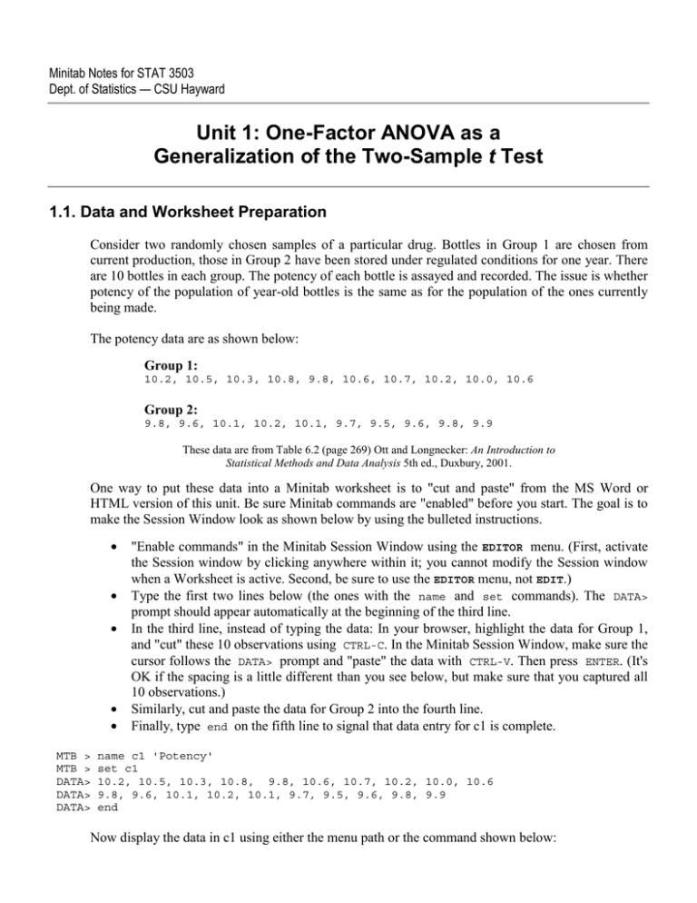
make the Session Window look as shown below by using the bulleted instructions.
•
•
•
•
•
MTB >
MTB >
DATA>
DATA>
DATA>
"Enable commands" in the Minitab Session Window using the EDITOR menu. (First, activate
the Session window by clicking anywhere within it; you cannot modify the Session window
when a Worksheet is active. Second, be sure to use the EDITOR menu, not EDIT.)
Type the first two lines below (the ones with the name and set commands). The DATA>
prompt should appear automatically at the beginning of the third line.
In the third line, instead of typing the data: In your browser, highlight the data for Group 1,
and "cut" these 10 observations using CTRL-C. In the Minitab Session Window, make sure the
cursor follows the DATA> prompt and "paste" the data with CTRL-V. Then press ENTER. (It's
OK if the spacing is a little different than you see below, but make sure that you captured all
10 observations.)
Similarly, cut and paste the data for Group 2 into the fourth line.
Finally, type end on the fifth line to signal that data entry for c1 is complete.
name c1 'Potency'
set c1
10.2, 10.5, 10.3, 10.8, 9.8, 10.6, 10.7, 10.2, 10.0, 10.6
9.8, 9.6, 10.1, 10.2, 10.1, 9.7, 9.5, 9.6, 9.8, 9.9
end
Now display the data in c1 using either the menu path or the command shown below:
Minitab Notes for STAT 3503
Unit 1-2
DATA (MANIP in Releases 13 and earlier) ➯ Display Data
MTB > print c1
This produces a (horizontal) printout of the 20 observations in c1. Also look in the worksheet to see
the data there.
Next we need a column of "subscripts" in c2 to show which observations come from which group.
Name c2 'Group' either with a command or by typing the name directly into the worksheet. Then
enter the subscripts using either the menus (bold type) or the set command.
Type Group atop column 2 in the Worksheet
CALC ➯ Patterned Data, Simple, values from 1 to 2,
each individual value repeated 10 times
MTB > name c2 'Group'
MTB > set c2
DATA> (1:2)10
DATA> end
This way of organizing data, with all observations in a single column and groups designated in a
separate column of subscripts, is called "stacked" format.
For such a small dataset you could just type the 20 'Potency' determinations and the 20 'Group'
numbers directly into the worksheet. However, when using documents in DOC or HTML format, you
may find it convenient to learn (i) to cut and paste data into a worksheet and (ii) to use the "patterned
data" features of the set command. It is best to start learning with the current relatively simple data
to do these two things.
Once you have entered data into a worksheet, you should always proofread your work before
continuing. You can do this either by printing the data to the Session window (using the print
command) or by looking directly at the Worksheet. Proofreading should become an automatic part of
data entry for you. Beyond the first few units these notes will not remind you to do this.
Problems
1.1.1. Here is an alternate way to prepare the worksheet. Follow through the steps, cutting and pasting
data where appropriate. What menu choices would produce the same results? [Look at the DATA
(MANIP) menu.] Explain what each command does. Compare c13 and c14 with c1 and c2.
MTB >
MTB >
DATA>
DATA>
MTB >
DATA>
DATA>
MTB >
SUBC>
name c11 'Fresh' c12 'Stored'
set c11
10.2, 10.5, 10.3, 10.8, 9.8, 10.6, 10.7, 10.2, 10.0, 10.6
end
set c12
9.8, 9.6, 10.1, 10.2, 10.1, 9.7, 9.5, 9.6, 9.8, 9.9
end
stack c11 c12 c13;
subs c14.
1.1.2. In the process of working Problem 1.1.1 you put the data for each group into a separate column
(c11 and c12). Data in separate columns are said to be in "unstacked" format. Look at the DATA
(MANIP) menu and figure out how the stacked data in c1 can be put into unstacked format using the
subscripts in c2. (Use the column names c21 'New' and c22 'Old' for this.) What command/
subcommand combination could you use to unstack the data, without the help of the menus? (Minitab
is a command-based package. The menus are sometimes a convenient way to generate commands,
which appear in the Session window when the command language is active.)
Minitab Notes for STAT 3503
Unit 1-3
1.2. Descriptive Methods
Whenever possible, data analysis should begin with descriptive methods, both numerical and
graphical. Here, it seems clear from the dotplot that the potency of the stored bottles is less than the
potency of the fresh ones: Group 1 (mean above 10.25) has generally higher values than Group 2
(mean below 10.00).
PLOT ➯ Character ➯ Dotplot, by variable
MTB > gstd
MTB > dotp c1;
SUBC> by c2.
Group
1
.
.
:
.
.
:
.
.
---+---------+---------+---------+---------+---------+---Potency
Group
2
.
:
.
:
.
:
.
---+---------+---------+---------+---------+---------+---Potency
9.50
9.75
10.00
10.25
10.50
10.75
Now we compute numerical descriptive statistics broken out, by the subscript variable in c2, into two
groups.
STAT ➯ Basic ➯ Descriptive statistics, by variable
MTB > describe c1;
SUBC> by c2.
Variable
Potency
Group
1
2
N
10
10
N*
0
0
Variable
Potency
Group
1
2
Q3
10.625
10.1000
Mean
10.370
9.8300
SE Mean
0.102
0.0761
StDev
0.323
0.2406
Minimum
9.800
9.5000
Q1
10.150
9.6000
Median
10.400
9.8000
Maximum
10.800
10.2000
Note: The printout above was made using Release 14; Release 13 produces a slightly different
result.
Problems
1.2.1. Minitab makes graphical displays in one of two formats:
• Standard (or Character) graphics. These are composed of text symbols and appear in the
Session window. They have relatively low resolution, but they are easy to paste into reports
using a work processor. (Be sure to use a monospace font such as Courier and to proofread to
make sure the graph looks the same after pasting as it did before cutting from Minitab.) They
are also quick and convenient to transmit over the web. We mainly show standard graphics in
these notes. To activate standard graphics, use the command gstd and then issue the
command for the kind of graph desired. Alternatively, select a character graphic from the
GRAPH menu.
• Professional (or Pixel) graphics. These are true graphic images using Windows technology.
They appear in separate boxes on your screen, not in the Session window. These images can
be saved in a variety of graphics formats, some of which can be edited with graphics software.
Minitab Notes for STAT 3503
Unit 1-4
They can be included as graphic images on the web and can be imported into word processing
and desk-top publishing documents. They greatly increase the file size of documents that
incorporate them. Minitab starts in professional graphics mode. To re-activate professional
graphics after using character graphics, use the command gpro.
Illustrate both types of graphics by making boxplots as follows:
MTB > gstd
MTB > boxp c1;
SUBC> by c2.
MTB > gpro
MTB > boxp c1 * c2
MTB > dotp c1 * c2
Comment on the results as follows:
(a) Do the boxplots show the differences between the two groups as clearly as do the
dotplots? More clearly? Defend your answer.
(b) Look at one of the dotplots above. Can you see exactly how many data points are
represented? Now look at one of the boxplots above. Can you see how many data
points are represented?
(c) Minitab's boxplots sometimes indicate the presence of outliers. Are outliers
indicated for either of our groups?
(d) What descriptive statistics are used in making box plots?
(e) Comment on the differences between standard-graphics and professional-graphics
boxplots.
(f) We have given several commands above. What menu choices can be used to
produce each style of boxplot?
1.3. t Test and One-Factor ANOVA
The descriptive methods in Section 1.2 strongly suggest that fresh samples of the drug tend to be
more potent than stored ones. Now we look at several different ways to confirm this impression with
formal statistical tests. That is, we test H0: the 2 groups have equal potency against Ha: the 2 groups
have different potencies.
The first of these is the two-tailed, pooled two-sample t test. The command for a two-sample t test on
stacked data is twot.
Minitab defaults for two-sample t tests:
•
•
The two-tailed alternative is the default; one-sided alternatives require the subcommand
alternative followed by either 1 (right-sided alternative) or -1 (left-sided).
The separate variances ("t-prime") test is the default. Pooling requires the subcommand pool.
Computer simulation results have established that the separate variances test is often
preferable for two-sample tests. Here we use the pooled test because it generalizes more
readily to the ANOVA methods of these notes.
Minitab Notes for STAT 3503
Unit 1-5
Note on stacked vs. unstacked data: The command twosample would be used if
the potency measurements for the two groups had been entered into two separate
columns--one for Fresh and one for Stored. Such "unstacked" data are seldom used
for computer analysis outside of elementary statistics classes. Minitab is one of the
few serious computer packages that makes direct use of unstacked data--and, even
then, only for a few elementary procedures.
STAT ➯ Basic ➯ 2-sample t, one column, assume equal variances
MTB > twot c1 c2;
SUBC> pool.
Two-sample T for Potency
Group
1
2
N
10
10
Mean
10.370
9.830
StDev
0.323
0.241
SE Mean
0.10
0.076
Difference = mu (1) - mu (2)
Estimate for difference: 0.540000
95% CI for difference: (0.272230, 0.807770)
T-Test of difference = 0 (vs not =): T-Value = 4.24
Both use Pooled StDev = 0.2850
P-Value = 0.000
DF = 18
We see (from the very small P-value) that the difference between the two groups is very highly
significant. This is what we guessed would be the case from looking at the dotplots above. Either the
Fresh samples were manufactured to have a higher potency or the potency of the Stored samples
deteriorated with a year of storage.
The one-factor or one-way ANOVA design (also sometimes called the "completely randomized
design") is a generalization of the two-sided, pooled two-sample t test that can handle more than two
groups. Thus, when it is applied to only two groups, its result should agree with that of the t test.
STAT ➯ ANOVA ➯ Oneway
MTB > oneway c1 c2
(Alternatively:
MTB > onew 'Potency' 'Group')
One-way ANOVA: Potency versus Group
Source
Group
Error
Total
DF
1
18
19
S = 0.2850
Level
1
2
N
10
10
SS
1.4580
1.4620
2.9200
MS
1.4580
0.0812
R-Sq = 49.93%
Mean
10.370
9.830
StDev
0.323
0.241
F
17.95
P
0.000
R-Sq(adj) = 47.15%
Individual 95% CIs For Mean Based on
Pooled StDev
----+---------+---------+---------+----(-------*------)
(------*-------)
----+---------+---------+---------+----9.75
10.00
10.25
10.50
Pooled StDev = 0.285
Note: Releases 13 and earlier omit some of the information shown in this Release 14 printout.
Minitab Notes for STAT 3503
Unit 1-6
The P-value for both the t test and the one-way ANOVA is 0.00049. Depending on the release of
Minitab this may be printed as 0.000 (meaning less than 0.0005) or rounded to 0.0005.
The square of a t-distributed random variable with 18 df is an F-distributed random variable with 1 df
in the numerator and 18 df in the denominator. In fact, the squares of the .025 values for t(ν) are the
.05 values for F(1, ν), as you can verify by looking at tables. [Upon squaring, the negative (left) and
positive (right) tails of t both go into the right tail of F: .025 + .025 = .05.]
Also, the square of the t-statistic obtained in our t test above is the F-statistic in our ANOVA:
4.242 = 17.95.
Note: In Minitab, the oneway procedure is the simplest of several ways to perform a
one-way ANOVA on stacked data. This command requires column identifiers such as c1 and c2,
or 'Potency' and 'Group' (column names inside single quotes). It does only one-way ANOVAs,
and provides separate confidence intervals for each level (Fresh or Stored) of the single factor
(Group).
Problems:
1.3.1. For a two-sample design with n = 10 observations in each group and a fixed significance level
α = .05, find the critical values for the two-sided pooled t test and the F test discussed above. Use
Minitab's invcdf command:
MTB > invcdf 0.975;
SUBC> t 18.
MTB > invcdf 0.95;
SUBC> F 1 18.
Compare your results with tables in your text. Verify that the square of the critical value for t is the
critical value for F. In this problem, why do you need to use y = 0.975 for the t distribution and 0.95
for the F distribution? (For each distribution, draw a sketch and shade in the area corresponding to
probability 0.05.)
[Recall that the cumulative distribution function (cdf) F(x) of a random variable X is P(X < x). Thus,
the inverse cdf function for a particular value y gives the value c such that P(X < c) = y. The inverse
cdf function is sometimes called the quantile function.]
1.3.2. Consider a balanced two-sample design in which each group has n observations. Let the group
totals be T1 and T2, and denote the grand total of all observations as T1 + T2 = G. Express the formulas
for both the pooled t-statistic and the F-statistic discussed above in terms of this notation. Then use
simple algebra to verify that the F-statistic is the square of the t-statistic.
1.4. More-General Procedures
Minitab's general anova procedure will handle a great variety of ANOVA models, many of which
we shall study in these notes.
•
With commands: designate the response variable (Potency here), followed by an equal sign,
followed by the design or independent variables containing subscripts (here only one,
Minitab Notes for STAT 3503
•
Unit 1-7
'Group'). Use of single quotes (apostrophes) around variable names is optional (unless the first
character of the name is a number or a symbol).
With Windows menus: you must select the response variable in one dialog box and the
subscript variables that specify the model in another. (For now, ignore the box for "random"
factors.)
For more complicated designs than the completely randomized design, ANOVA will handle only
balanced situations, i.e., only designs where each treatment (or treatment combination) has the same
number of replications. Because it is programmed to handle such a wide variety of ANOVA designs,
the general ANOVA procedure does not provide confidence intervals.
STAT ➯ ANOVA ➯ Balanced, select 'Potency' as Response, 'Group' as Model
MTB > anova Potency = Group
Factor
Group
Type
fixed
Levels
2
Values
1, 2
Analysis of Variance for Potency
Source
Group
Error
Total
DF
1
18
19
S = 0.284995
SS
1.4580
1.4620
2.9200
MS
1.4580
0.0812
R-Sq = 49.93%
F
17.95
P
0.000
R-Sq(adj) = 47.15%
Finally, the GLM procedure (stands for "general linear model") has the same syntax as ANOVA. It
requires more intensive computation and more computer memory (perhaps noticeable with large
datasets and complex designs), can handle unbalanced cases, uses a regression approach, and
automatically warns us about "unusual" observations. For more complex designs the two procedures
have somewhat different options and capabilities.
STAT ➯ ANOVA ➯ General linear model
MTB > glm Potency = Group
Factor
Group
Levels Values
2
1
2
Analysis of Variance for Potency
Source
Group
Error
Total
DF
1
18
19
S = 0.284995
Seq SS
1.4580
1.4620
2.9200
R-Sq = 49.93%
Adj SS
1.4580
1.4620
Adj MS
1.4580
0.0812
F
17.95
P
0.000
R-Sq(adj) = 47.15%
Unusual Observations for Potency
Obs.
5
Potency
9.8000
Fit Stdev.Fit
10.3700
0.0901
Residual
-0.5700
St.Resid
-2.11R
R denotes an obs. with a large st. resid.
Technical note: Because Group and Error correspond to orthogonal subspaces of the
20-dimensional vector space of observations, the Sequential and Adjusted Sums of
Squares are identical for our data.
Minitab Notes for STAT 3503
Unit 1-8
Problems:
1.4.1. The GLM procedure indicates that observation #5 is unusual. Minitab's criterion for calling an
observation unusual is based on Studentized residuals of absolute value greater than 2. So this
observation with its value of -2.11 is borderline. (We will not go into the computations involved in
finding Studentized residuals. Very roughly, the idea is that this observation is relatively far from the
mean of the rest of the observations in its group.)
In this ANOVA, the (ordinary) residual of an observation is its difference from its group means.
Using menus, in the one-way ANOVA procedure select the option to store residuals. Verify the
values of the residuals for observations #1, #5, and #11 of the stacked data by hand. Make a box plot
of the residuals. Does it indicate any outliers?
1.4.2. Use the menu path STAT ➯ Basic statistics ➯ Normality test to test the null
hypothesis that the residuals fit a normal distribution (against the alternative that they are not
normal). In the resulting normal probability plot, normal residuals should nearly fit a straight line. Do
ours? What is the P-value of the Anderson-Darling test of normality?
1.4.3. Test the hypothesis that the two groups come from populations with equal variances against
the two-sided alternative. Use the cdf command to find the P-value of this test. (The Fmax-test for t
treatment groups is equivalent to the F test if t = 2. Verify this for the Potency data. Tables of the
Fmax-distribution are available in Ott/Longnecker, and in some other texts. )
1.5. Nonparametric Alternatives
Here we mention several nonparametric tests. You should read the descriptions of them in your
text. In Windows, all menu paths for Minitab's implementations of these tests begin with
STAT > Nonparametric.
•
•
The nonparametric alternative to the two-sample t test is the Mann-Whitney-Wilcoxon test
(command mann). It works only for unstacked data.
Both of the nonparametric alternatives to the general one-way ANOVA are programmed to be
used with stacked data: the Mood test (Minitab command mood) and the Kruskal-Wallis test
(Minitab command kruskal). The Kruskal-Wallis test is a generalization of the MannWhitney-Wilcoxon test in the same sense that the one-way ANOVA is a generalization of a
pooled two-sample t test.
Unlike the t test and ANOVA, none of these nonparametric tests assume normal data. They all test
null hypotheses about equal population medians (rather than means).
Like their normal-theory counterparts, these nonparametric tests assume that:
•
•
•
The data are random samples from their respective populations,
The data for different levels (e.g., Fresh and Stored groups) are independent of one another,
The population dispersions are equal. For the normal tests, the specific form of the "equal
dispersion" assumption is that variances are equal. For the nonparametric tests, it is that all
population distributions are of the same shape, differing (if at all) only by a translation that
shifts the entire distribution along with the value of the median.
Minitab Notes for STAT 3503
•
Unit 1-9
The populations are continuous to the extent necessary to avoid "ties" (repeated values).
Normal theory tests usually work quite well unless rounding (or some other process) has
produced severe granularity (many clumps of repeated values. Nonparametric tests require
approximate "correction" procedures to adjust for any ties that may be present due to
rounding.
There is no evidence that our present data are other than normally distributed. For example, the
dotplots and boxplots show no marked skewness or probable outliers. Even so, you should
experiment with the nonparametric procedures kruskal and mood to see how they work. Here,
they yield the same conclusion as the normal theory tests: the potency of the stored bottles is less than
for the fresh ones.
Problems:
1.5.1. Theoretically, for continuous data there should be no ties at all. In reality, we are always
dealing with rounded data, so ties may be present. (For example, truly distinct values 10.1990213 and
10.2037681 would both be recorded here as "tied" at 10.2; even with two-decimal accuracy both
would be recorded as 10.20. ) Looking at the 20 observations in our dataset, do you find any ties? If
so, how many observations are involved in ties?
1.5.2. The W-statistic reported in the output of Minitab's implementation mann of the MannWhitney-Wilcoxon test is computed as follows: consider all of the data in both groups as a whole,
find the ranks of these observations, and find the sum of the ranks of the observations in Group 1. A
small value of W indicates that Group 1 comes from a population with a smaller median than
Group 2; a large value indicates that the population median for Group 1 may be larger.
(a) Under the null hypothesis that the two populations are the same, the expected value
of W can be shown to be µW = n1(n1 + n2 + 1)/2. What is this value for our data?
(b) Assume that c5, c6, and c7 are empty columns, that the stacked data are in c1 and
that the subscripts are in c2. The following Minitab commands can be used to illustrate
how W is computed:
MTB >
MTB >
SUBC>
MTB >
rank c1 c5
unstack c5 c6 c7;
subs c2.
sum c6.
Go through these steps carefully, looking at the worksheet after each step and making
sure you understand what each step does. Then unstack the data and use the mann
command to perform the Mann-Whitney-Wilcoxon test. Compare the value of W with
your computations above. Carefully compare the interpretation of this nonparametric
test with the interpretation of the t test and the ANOVA above? Justify your answer.
Minitab Notes for Statistics 3503 by Bruce E. Trumbo,
Department of Statistics, CSU Hayward, Hayward CA, 94542,
Email: btrumbo@csuhayward.edu.
Comments and corrections welcome.
Copyright © 1991, 1995, 1997, 1998, 2000, 2001, 2002, 2004 by Bruce E. Trumbo. All rights reserved. These notes are intended
for use at CSU Hayward in classes where Ott/ Longnecker is a required text. Please contact the author at the address above to
request permission for other uses. Preparation of early versions of these notes was partially supported by NSF grant USE-9150433.
Revised 1/2004.