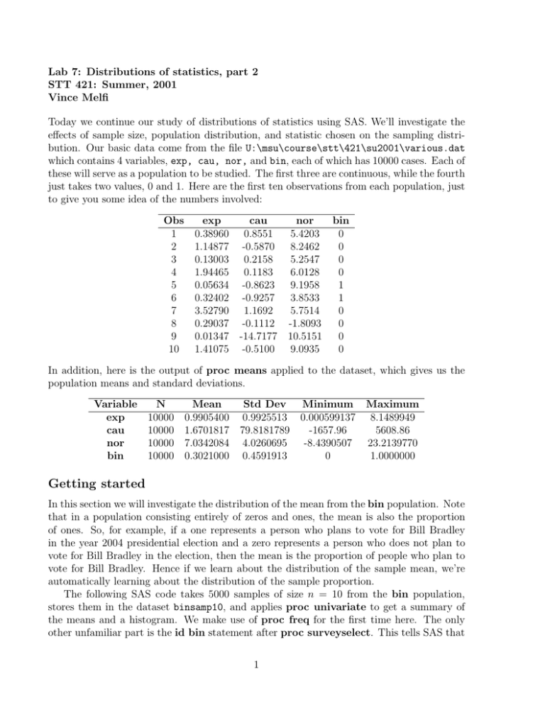
Lab 7: Distributions of statistics, part 2
STT 421: Summer, 2001
Vince Melfi
Today we continue our study of distributions of statistics using SAS. We’ll investigate the
effects of sample size, population distribution, and statistic chosen on the sampling distribution. Our basic data come from the file U:\msu\course\stt\421\su2001\various.dat
which contains 4 variables, exp, cau, nor, and bin, each of which has 10000 cases. Each of
these will serve as a population to be studied. The first three are continuous, while the fourth
just takes two values, 0 and 1. Here are the first ten observations from each population, just
to give you some idea of the numbers involved:
Obs
1
2
3
4
5
6
7
8
9
10
exp
cau
0.38960 0.8551
1.14877 -0.5870
0.13003 0.2158
1.94465 0.1183
0.05634 -0.8623
0.32402 -0.9257
3.52790 1.1692
0.29037 -0.1112
0.01347 -14.7177
1.41075 -0.5100
nor
bin
5.4203
0
8.2462
0
5.2547
0
6.0128
0
9.1958
1
3.8533
1
5.7514
0
-1.8093
0
10.5151
0
9.0935
0
In addition, here is the output of proc means applied to the dataset, which gives us the
population means and standard deviations.
Variable
exp
cau
nor
bin
N
10000
10000
10000
10000
Mean
0.9905400
1.6701817
7.0342084
0.3021000
Std Dev
0.9925513
79.8181789
4.0260695
0.4591913
Minimum Maximum
0.000599137 8.1489949
-1657.96
5608.86
-8.4390507 23.2139770
0
1.0000000
Getting started
In this section we will investigate the distribution of the mean from the bin population. Note
that in a population consisting entirely of zeros and ones, the mean is also the proportion
of ones. So, for example, if a one represents a person who plans to vote for Bill Bradley
in the year 2004 presidential election and a zero represents a person who does not plan to
vote for Bill Bradley in the election, then the mean is the proportion of people who plan to
vote for Bill Bradley. Hence if we learn about the distribution of the sample mean, we’re
automatically learning about the distribution of the sample proportion.
The following SAS code takes 5000 samples of size n = 10 from the bin population,
stores them in the dataset binsamp10, and applies proc univariate to get a summary of
the means and a histogram. We make use of proc freq for the first time here. The only
other unfamiliar part is the id bin statement after proc surveyselect. This tells SAS that
1
we only want samples from the bin population, not the others. Run the program and then
use the output to answer the questions below.
NOTE: To save space, I haven’t included any title statements in the SAS programs. It
would be wise to add title statements to your programs to keep track of the copious
output! Also, the programs will take a few (maybe 20–30) seconds to run.
data various;
infile ’u:\msu\course\stt\421\su2001\various.dat’;
input exp cau nor bin;
proc surveyselect data = various n = 10 rep = 1000 out = binsamp10;
id bin;
proc univariate data = binsamp10 noprint;
output out = binmeans10 mean = Mean;
var bin;
by replicate;
proc univariate data = binmeans10;
var mean;
histogram mean / midpoints = 0 to 1 by 0.1;
proc freq data = binmeans10;
run;
Explanation
Here’s an explanation of some parts of the SAS program.
1. In the proc surveyselect statement, we specify the dataset to sample from via
data=various, the sample size via n = 10, the number of times to repeat the sampling
procedure via rep = 1000, the dataset to store the samples in via out = binsamp10,
and the variable to sample from via id bin.
2. In the first proc univariate statement we request no output1 via noprint, we request that the means be stored in a dataset called binmeans10 via output out =
binmeans10 mean = Mean, we specify the variable we want to apply proc univariate to via var bin,2 and we specify that we want separate means for each sample
via by replicate.
1
Otherwise we’d have reams of output since we ask for a separate computation for each of the 1000
replicates.
2
The proc surveyselect procedure automatically called the variable containing the samples bin.
2
3. Because the mean of each sample will be one of the numbers 0, 0.1, 0.2, ...,
0.9, 1, we specify that we’d like the midpoints of the histogram intervals to be at
these values via midpoints = 0 to 1 by 0.1.
4. The proc freq statement requests a frequency table of the 1000 means. Look at the
output to see what you get. You’ll find this useful in answering some of the questions
below.
Questions
Here are some questions to answer. Note that the population proportion of ones is 0.3 (you
can check this via proc means if you’d like), so we’d be happy with an estimate that’s close
to 0.3. (Of course in a realistic setting we’d not know this true value.)
1. What is the mean of the 1000 sample means?
2. What is the standard deviation√
of the 1000 sample means? Is it close to the population
standard deviation divided by n?
3. What proportion of the 1000 sample means are within 0.1 of 0.3? (Count 0.2 and 0.4
as being within 0.1 of 0.3.)
4. What proportion of the 1000 sample means are within 0.05 of 0.3?
5. What proportion of the 1000 sample means are within 0.02 of 0.3?
6. Is the histogram of sample means reasonably symmetric and bell-shaped?
Increasing the sample size
Now we’ll see how the distribution of the sample mean (which in this case is also the sample
proportion) changes when we increase the sample size from n = 10 to n = 50. The SAS code
is below. Note that (as long as you’re in the same SAS session) you can leave out the initial
data various;
infile ’u:\msu\course\stt\421\su2001\various.dat’;
input exp cau nor bin;
since the various dataset is already loaded into SAS. This will make your program run a
bit quicker. Note also that the program is very similar to the n = 10 program. Mainly we
replace 10 by 50 throughout that program, and also change the midpoints of the histogram
slightly.
proc surveyselect data = various n = 50 rep = 1000 out = binsamp50;
id bin;
proc univariate data = binsamp50 noprint;
output out = binmeans50 mean = Mean;
3
var bin;
by replicate;
proc univariate data = binmeans50;
var mean;
histogram mean / midpoints = 0 to 1 by 0.05;
proc freq data = binmeans50;
run;
Questions
1. What is the mean of the 1000 sample means?
2. What is the standard deviation√
of the 1000 sample means? Is it close to the population
standard deviation divided by n?
3. What proportion of the 1000 sample means are within 0.1 of 0.3? (Count 0.2 and 0.4
as being within 0.1 of 0.3.)
4. What proportion of the 1000 sample means are within 0.05 of 0.3?
5. What proportion of the 1000 sample means are within 0.02 of 0.3?
6. Is the histogram of sample means reasonably symmetric and bell-shaped? How does
it differ from the histogram from n = 10?
Increasing the sample size
Repeat the procedure, this time with a sample size of n = 250. Again answer the questions:
1. What is the mean of the 1000 sample means?
2. What is the standard deviation√
of the 1000 sample means? Is it close to the population
standard deviation divided by n?
3. What proportion of the 1000 sample means are within 0.1 of 0.3? (Count 0.2 and 0.4
as being within 0.1 of 0.3.)
4. What proportion of the 1000 sample means are within 0.05 of 0.3?
5. What proportion of the 1000 sample means are within 0.02 of 0.3?
6. Is the histogram of sample means reasonably symmetric and bell-shaped? How does
it differ from the histograms from n = 10 and n = 50?
4
Another population
Next we look at the distributions of the sample mean and sample median from a different
population, contained in the variable nor. This population is a nice, symmetric population
with mean and median both equal to about 7. We start with n = 5.
proc surveyselect data = various n = 5 rep = 1000 out = norsamp5;
id nor;
proc univariate data = norsamp5 noprint;
output out = normeans5 mean = Mean;
var nor;
by replicate;
proc univariate data = norsamp5 noprint;
output out = normeds5 median = Median;
var nor;
by replicate;
proc univariate data = normeans5;
var mean;
histogram mean;
proc univariate data = normeds5;
var median;
histogram median;
run;
Questions
1. What is the mean of the 1000 sample means? Is it close to the population mean?
2. What is the standard deviation√
of the 1000 sample means? Is it close to the population
standard deviation divided by n?
3. What is the median of the 1000 sample means? Is it close to the population mean?
4. What is the standard deviation of the 1000 sample medians? Is it larger or smaller
than the standard deviation of the 1000 sample means?
5. Is the histogram of sample means reasonably symmetric and bell-shaped?
6. Is the histogram of sample medians reasonably symmetric and bell-shaped?
5
Rasing the sample size
Repeat the above simulation with n = 75 rather than n = 5. Answer the following questions.
1. What is the mean of the 1000 sample means? Is it close to the population mean?
2. What is the standard deviation√
of the 1000 sample means? Is it close to the population
standard deviation divided by n?
3. What is the median of the 1000 sample means? Is it close to the population mean?
4. What is the standard deviation of the 1000 sample medians? Is it larger or smaller
than the standard deviation of the 1000 sample means?
5. Is the histogram of sample means reasonably symmetric and bell-shaped?
6. Is the histogram of sample medians reasonably symmetric and bell-shaped?
Yet another population
For the population contained in the variable exp, repeat the above simulation involving the
mean and median with n = 5. Answer the following questions.
1. What is the mean of the 1000 sample means? Is it close to the population mean?
2. What is the mean of the 1000 sample medians? Is it close to the population mean?
Can you explain why it is not? (Hint: You may want to look at a histogram of the
population.)
3. Is the histogram of sample means reasonably symmetric and bell-shaped?
4. Is the histogram of sample medians reasonably symmetric and bell-shaped?
6