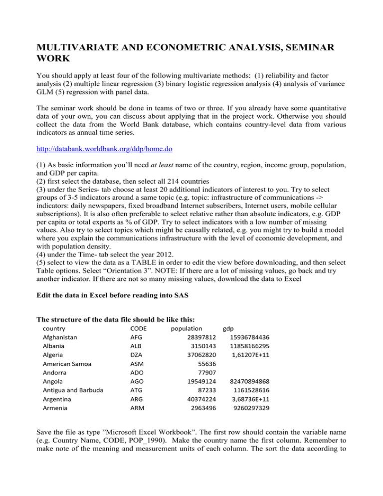
MULTIVARIATE AND ECONOMETRIC ANALYSIS, SEMINAR
WORK
You should apply at least four of the following multivariate methods: (1) reliability and factor
analysis (2) multiple linear regression (3) binary logistic regression analysis (4) analysis of variance
GLM (5) regression with panel data.
The seminar work should be done in teams of two or three. If you already have some quantitative
data of your own, you can discuss about applying that in the project work. Otherwise you should
collect the data from the World Bank database, which contains country-level data from various
indicators as annual time series.
http://databank.worldbank.org/ddp/home.do
(1) As basic information you’ll need at least name of the country, region, income group, population,
and GDP per capita.
(2) first select the database, then select all 214 countries
(3) under the Series- tab choose at least 20 additional indicators of interest to you. Try to select
groups of 3-5 indicators around a same topic (e.g. topic: infrastructure of communications ->
indicators: daily newspapers, fixed broadband Internet subscribers, Internet users, mobile cellular
subscriptions). It is also often preferable to select relative rather than absolute indicators, e.g. GDP
per capita or total exports as % of GDP. Try to select indicators with a low number of missing
values. Also try to select topics which might be causally related, e.g. you might try to build a model
where you explain the communications infrastructure with the level of economic development, and
with population density.
(4) under the Time- tab select the year 2012.
(5) select to view the data as a TABLE in order to edit the view before downloading, and then select
Table options. Select “Orientation 3”. NOTE: If there are a lot of missing values, go back and try
another indicator. If there are not so many missing values, download the data to Excel
Edit the data in Excel before reading into SAS
The structure of the data file should be like this:
country
Afghanistan
Albania
Algeria
American Samoa
Andorra
Angola
Antigua and Barbuda
Argentina
Armenia
CODE
AFG
ALB
DZA
ASM
ADO
AGO
ATG
ARG
ARM
population
gdp
28397812
15936784436
3150143
11858166295
37062820
1,61207E+11
55636
77907
19549124
82470894868
87233
1161528616
40374224
3,68736E+11
2963496
9260297329
Save the file as type ”Microsoft Excel Workbook”. The first row should contain the variable name
(e.g. Country Name, CODE, POP_1990). Make the country name the first column. Remember to
make note of the meaning and measurement units of each column. The sort the data according to
CODE to ascending order. Initially you should do a separate Excel sheet for each indicator, and later
on you can combine the different indicators into the same sheet either in Excel or in SAS. Make sure
that the rows match so that in the combined file all indicators for a certain country are in the same
row. If you have used different databases there can be different countries included and then the rows
do not automatically match.
Another way is to combine the files in SAS:
Read each Excel file into SAS:
The first row of the Excel-sheet must contain variable names and the data must begin from row 2.
1. Open SAS Enterprise Guide.
2. Choose New project
3. Define the library reference by selecting File –New –Code and type into the new window:
Libname somename BASE ’directorypath’;
Somename is the name you assign for the library, e.g. MAIJA, and the path to your folder is inside
the hyphens. Your folder is either in a memory stick (E: F:) or your home directory (Z:) . After typing,
save this code by choosing File- Save Code As… -Local Computer and run it by clicking on the icon
with the right mouse button and choosing Run libreference On Local.
Now you can bring in the Excel file: File- Import Data- Local Computer. ”Import Data” window
opens and ”Region to Import” –sheet lets you specify the range to import.
Use this to bring all data
Variable names on this
row
”Colum Options” –sheet allows you to check that the type of variables is correct (mostly numeric)
and to type in descriptive labels for the variable names.
”Results” –sheet lets you specify where to save the file. Click Browse and choose Libraries from the
drop-down menu.
Open your own library reference name, which you specified in the beginning of the SAS session.
Enter a filename and click Save.
Then select Run and you SAS data file opens up.
Then repeat these data importing steps until you have all the excel-files imported and saved as
separate SAS-datafiles (named as maija.esimerkki1, maija.esimerkki2, etc.). All these separate
datafiles should have Country Name as the first variable, CODE as the second variable and different
other variable names. In the upper left corner, Choose create new item in project – code and type
the following:
data maija.newcombined;
merge maija.esimerkki1 maija.esimerkki2 maija.esimerkki3;
by CODE;
proc print data = newcombined;
run;
REPORT
-
Title page should include: title of the project, date, authors’ names, authors’ student numbers
Table of contents
-
1.
2.
3.
4.
5.
6.
7.
8.
Use page numbering. Figures and Tables should all have a number and title. They should be
referred to in the text.
Font size 12, line spacing 1.5, margins 2-3 cm
Total length of the report about 20 – 40 pages + appendices
Tables and graphs can be copied from SAS output to your report, but often it is useful to
combine information from several SAS output tables into a single one. Very large or less
important tables and graphs can be included as appendices.
Appendices should be numbered and titled and referred to in the text.
Literature references mainly related to methodology, no theory references needed
Harvard style referencing
grading 75% written report and 25% presentation
DL 29.3.2015, at 23.59, return to kaisu.puumalainen@lut.fi
Structure of the report for example as follows:
INTRODUCTION
- Purpose of the study
- Research questions and main concepts
- Data collection
- Analysis methods
DESCRIPTIVE ANALYSIS
- Graphs, distributions, descriptive statistics of the main variables, preferably also by
some basic categorization like like region or income group
- Data transformations, e.g. , categorizations, logs or per capita transformations
MEASURE DEVELOPMENT
- factor analyses and reliabilities
- descriptive analysis of the developed measures
EXPLANATORY ANALYSIS
- This section can be grouped either by research questions or analysis methods used
- Methods e.g. correlation, crosstabs, t- tests, regression and variance analyses
CONCLUSIONS
- Main results and discussion of their meaning/implications
- Evaluation of validity, limitations
- Ideas for further research
REFERENCES
APPENDICES
- E.g. correlation matrices, histograms, residual or influence plots
PANEL DATA DESCRIPTION AND REGRESSION ANALYSIS
PRESENTATION
-
13.4.2015
Each presentation should last about 10 - 15 minutes
Use powerpoint, and bring your file on a memory stick
Participation in the seminar is mandatory unless you do the project work alone
Presentations are graded jointly by the participants
Presentation grade is 25% of the final grade
GRADING OF THE WRITTEN REPORT
Introduction 0-5 p
Descriptive analysis 0-10 p
Measure development 0-10 p
Linear regression analysis 0-10 p
Panel data regression analysis 0-10 p
Logistic regression analysis 0-5 p
GLM 0-5 p
Conclusion 0-5 p
Reporting style 0-10 p (format of the report, use of tables, graphs, appendices, clarity, structure)
Data and models 0-5 p (amount of data used, selection of topics, and if the models make sense)
Total max 75 p
GRADING OF THE PRESENTATION
Each of the following are evaluated 0-5 (0=lacking, 1=very poor, 2= poor, 3= satisfactory, 4= good,
5= excellent)
A. presentation skills max 15 p
clarity of communication 0-5
use of tables & graphs & visual elements 0-5
use of time & structure of the presentation 0-5
B. analysis skills max 10 p
competence in data collection and analysis 0-5
interpretation of results and their implications 0-5
Total max 25 p