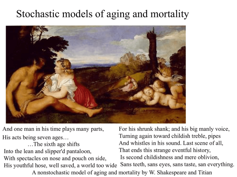
Stochastic models of aging and mortality
And one man in his time plays many parts,
For his shrunk shank; and his big manly voice,
Turning again toward childish treble, pipes
His acts being seven ages…
And whistles in his sound. Last scene of all,
…The sixth age shifts
That ends this strange eventful history,
Into the lean and slipper'd pantaloon,
Is second childishness and mere oblivion,
With spectacles on nose and pouch on side,
His youthful hose, well saved, a world too wide Sans teeth, sans eyes, sans taste, san everything.
A nonstochastic model of aging and mortality by W. Shakespeare and Titian
What is aging?
• J. M. Smith (1962): Aging processes are
“those which render individuals more
susceptible as they grow older to the various
factors, intrinsic or extrinsic, which may
cause death.”
• P. T. Costa and R. R. McCrae (1995): “What
happens to an organism over time.”
•“Force of mortality” (hazard rate) increases with
age
Increasing mortality as a proxy
for aging
• We can’t measure aging processes directly,
particularly since we can’t define them.
• Mortality rates are easy to measure. In most
metazoans, mortality rates increase with age.
Increasing mortality as a proxy
for aging
• We can’t measure aging processes directly,
particularly since we can’t define them.
• Mortality rates are easy to measure. In most
metazoans, mortality rates increase with age.
• This includes us.
This is not a trivial observation!
• Implicit in Roman annuity rates.
• 17th C. annuity and life-insurance rates
were generally age-independent.
• Annuity as gamble: Who is the best bet?
• Very old (for whom the increased hazard
would be most clear) rare, uncertain age.
• Extreme haphazardness of plagues, wars.
Some questions about aging:
1. Why do creatures age?
Some questions about aging:
1. Why do creatures age?
Old (and recurrent) idea:
Improper nutrition.
•“Unto the woman he said, I will
greatly multiply thy sorrow and thy
conception; in sorrow thou shalt
bring forth children; and thy desire
shall be to thy husband… In the
sweat of thy face shalt thou eat
bread, till thou return unto the
ground; for out of it wast thou
taken: for dust thou art, and unto
dust shalt thou return.”
Some questions about aging:
1. Why do creatures age?
THINGS FALL APART
Some questions about aging:
1. Why do creatures age?
Problems with this naïve answer
•Repair.
•Not universal.
Aging not universal.
• Negligible senescence: prokaryotes,
bristlecone pine, tortoises, lobster
• Gradual senescence: mammals, birds, fish,
yeast
• Rapid senescence: flies, bees (workers),
nematodes
Some questions about aging:
1. Why do creatures age?
2. Why does aging have the particular agepatterns that it does?
Some questions about aging:
1. Why do creatures age?
2. Why does aging have the particular agepatterns that it does?
3. Why do different species have
characteristic patterns of aging?
Some questions about aging:
1. Why do creatures age?
2. Why does aging have the particular agepatterns that it does?
3. Why do different species have
characteristic patterns of aging?
4. Why is aging so variable?
Some questions about aging:
1. Why do creatures age?
2. Why does aging have the particular agepatterns that it does?
3. Why do different species have
characteristic patterns of aging?
4. Why is aging so variable?
5. Why is aging so constant?
The Gompertz-Makeham
mortality law
• Gompertz (1825): “we observe that in those
tables the numbers of living in each yearly
increase of age are from 25 to 45 nearly, in
geometrical progression.”
• Makeham (1867): “Theory of partial forces
of mortality”. Diseases of lungs, heart,
kidneys, stomach, liver, brain associated
with “diminution of the vital power”.
log hazard rate in
Japan 1981-90
log infectious
disease
hazard rate in
Japan 1981-90
log cancer
hazard rate in
Japan 1981-90
log suicide
hazard rate in
Japan 1981-90
log auto accident
hazard rate in
Japan 1981-90
log breast cancer
hazard rate in
Japan 1981-90
log homicide
hazard rate in
Japan 1981-90
Species
Initial mort.
MRDT (yrs)
Max life (yrs)
Human (US F,
1980
.0002
8.9
122
Herring Gull
.0032
5.4
49
Horse
.0002
4
46
Rhesus monkey
.02
15
>35
Starling
.5
>8
20
Lake sturgeon
.013
10
>150
House fly
4-12
.02-.04
.3
Soil nematode
2
.02
.15
MRDT seems to be speciescharacteristic
Mortality plateaus
Female mortality at ages 80+ (Japan + 13 W. European countries (1980-92)
Mediterranean fruit fly mortality
Is this about biology?
“Force of junking” for automobiles
in various periods
Lifetimes of electrical relays
What is a Markov process?
A stochastic process Xt (where t is time,
usually taken to be the positive reals) such
that if you know the process up to a given
time t, the behavior after time t depends
only on the state at time t.
The process may be killed, either randomly (at
a rate depending on the current position) or
instantaneously when it hits a certain part of
the state space.
Lessons for young scientists from
reviewing the Markov mortality
model literature
• It’s easy to get your work published if
your model reproduces known
phenomena…
Lessons for young scientists from
reviewing the Markov mortality
model literature
• It’s easy to get your work published if
your model reproduces known
phenomena…
• … even if you put them in (decently
concealed) with your assumptions…
Lessons for young scientists from
reviewing the Markov mortality
model literature
• It’s easy to get your work published if
your model reproduces known
phenomena…
• … even if you put them in (decently
concealed) with your assumptions…
• … and even if the mathematics is
wrong.
“Challenge to homeostasis” (B.
Strehler, A. Mildvan 1960)
• “The rate of decrease of most physiologic
functions of human beings is between 0.5 and 1.3
percent per year after age 30, and is fit as well by
a straight line as by any other simple mathematical
function”.
• “Challenges” come at constant rate.
• Death occurs when a challenge exceeds the
organism’s “vital capacity”.
• “Challenges” follow the Maxwell-Boltzmann
distribution: Exponentially distributed.
“Challenge to homeostasis” (B.
Strehler, A. Mildvan 1960)
• “Predicts” the Gompertz curve.
• “Predicts” the “nonintuitive” fact that initial
mortality and rate of aging are inversely
related.
• Problem: The exponential rate was built into
the assumptions, for which there is no
external basis.
Extreme-value theory
• J. D. Abernethy (J. Theor. Biol. 1979): Model
organisms by independent “systems”, which all
fais at the same random rate. “Death” is the time
of the first failure.
• Proves that such an organism could have
exponentially increasing death rates.
• Claims (in the nonmathematical introduction and
conclusion) that this is the generic situation, which
will arise whenever the hazard rates of the
components are nondecreasing, which is untrue.
(In fact, the individual components would also
have to have exponential hazard rates.)
• Still gets cited.
Reliability theory
• M. Witten (1985): large number (m) of
critical components; death comes when all
fail.
• Components are independent. Fail with
constant rate.
• Derives hazard rate approximately
m·exp(t).
Reliability theory
• M. Witten (1985): large number (m) of
critical components; death comes when all
fail.
• Components are independent. Fail with
constant rate.
• Derives hazard rate approximately
m·exp(t).
• Unmentioned:  is negative, so the hazard
rate decreases exponentially
More reliability theory: Gavrilov &
Gavrilova (1990)
•
•
•
•
•
•
•
m critical organs, each with n redundant components.
Organ fails when all components fail.
Death comes when any organ fails.
Components fail independently with constant exponential rate.
Derive Weibull hazard rates (power law).
Want Gompertz hazard rates.
Declare that biological systems have most of their components
nonfunctioning from the beginning: Number of functioning
components in each organ is Poisson.
• The exponential of the Poisson then provides the exponential
hazard rates.
Biological problems with G&G
•
•
•
•
Arbitrary.
Where are the missing components?
What are the missing components?
Theory seems to predict that nearly all organisms
should be born dead, with Gompertz mortality
only conditioned on the rare survivors.
Small mathematical problem with G&G
model:
Big mathematical problem with G&G
model:
The computation is wrong.
Hazard rate for the
G & G series-parallel
process with k=1 and
==1 (solid) or
=2, =3 (dotted).
H. Le Bras’s “cascading failures”
model
•
•
•
•
Start at senescence state Xt=1.
Rate of jumps to next higher state is Xt.
Rate of dying is Xt.
Le Bras (1976) pointed out that when >>,
the mortality rate is about et for small t.
• True… but a little cheap. When >>, the
system behaves like a deterministic system
d Xt/dt= Xt. State is Xt et.
H. Le Bras’s “cascading failures”
model
• In fact, as Gavrilov & Gavrilova pointed out
(1990) the result is even better when you
don’t assume >>. By this time, mortality
plateaus had been recognized. The general
hazard rate is
(+)t
(+)t
-1
(+)e
(+e
) ,
which is a nice logistic Gompertz curve,
with plateau at +.
H. Le Bras’s “cascading failures”
model
• But… the exponential is still in the
assumptions.
• Also, the assumptions are quite
specific and arbitrary.
Attempts to explain the Gompertz
curve with Markov models have
been successful only when:
• The exponential increase was built
into the assumptions in a fairly
transparent way or
• The computations were wrong.
What about mortality plateaus?
Suggested explanations:
1. Heterogeneity in the population:
selection. (Analyzed in DS:
“Estimating mortality rate doubling time
doubling times”. Available as preprint.)
2. Individuals actually deteriorate more
slowly at advanced ages.
What about mortality plateaus?
• J. Weitz and H. Fraser (PNAS 2001) did
explicit computation for Brownian motion
with constant downward drift, killed at 0.
It shows “senescence” and “plateaus” -hazard rates increase rapidly (though not
exponentially) at first, but eventually
converge to a finite nonzero constant.
Criticisms of Weitz-Fraser
• The assumptions (constant diffusion rate, constant
downward drift, killing only at 0) are very specific.
• The assumptions have little empirical justification.
• The methods cannot be generalized to any other case.
Criticisms of Weitz-Fraser
• The assumptions (constant diffusion rate, constant
downward drift, killing only at 0) are very specific.
• The assumptions have little empirical justification.
• The methods cannot be generalized to any other case.
• For understanding anything other than the plateaus, the
model is too general: By choosing the starting distribution,
the hazard rate can become almost anything, as long as it
eventually converges to a rate ≤ b2/2. (Here b is the rate of
negative drift.)
In fact, the result is very general.
• Killed markov processes (which also may be
thought of as submarkov processes) converge
under fairly general conditions to quasistationary
distributions. That is,
The hazard rate will also converge to the rate
of killing in this distribution.
Some Theorems
• Let Xt be a diffusion on a one-dimensional interval
with drift b and variance 2, so satisfying the SDE
dXt= (Xt)dWt + b(Xt)dt,
and killed at the rate k(Xt). Let  be the smallest
such that there is a positive solution  to
()"—(b)'—k=—.
Some Theorems
• If both boundaries are regular then the distribution
of Xt,conditioned on survival converges to density
, and the mortality rate converges to .
• If ∞ is a natural or entrance boundary and r1
regular, then this convergence still holds if
(*)
• In the above, condition (*) may be replaced
by lim k(z)> .
z∞
Interpretation
• Mortality rates level off, not because the
process is changing, or because of selection
on populations with heterogeneous frailties.
The individuals who happen to survive a
long time simply tend to have a distribution
of vitality states which are somewhat spread
out, not arbitrarily piled up near points of
killing.
Why are there mortality-rate
plateaus?
Suggested explanations:
1. Heterogeneity in the population:
selection.
2. Individuals actually deteriorate more
slowly at advanced ages.
3. Those alive at advanced ages are, purely
by chance, inclined to be more fit than the
bare minimum required to stay alive.
For more information, see “Markov
mortality models: implications of
quasistationarity and varying initial
distributions” by DS and Steven
Evans. (Available as a preprint.)
Evolutionary theories
• Is mortality a trait shaped by natural
selection?
• No “overdesigned parts”.
• Medawar, Hamilton: Mutation-selection
equilibrium.
• Antagonistic pleiotropy.
• Kirkwood: Disposable soma.
Can evolutionary theory explain
Gompertz curve? Mortality plateaus?
• Charlesworth says yes to Gompertz.
• Mueller and Rose say yes to mortality
plateaus.
Charlesworth: Mutation-selection
equilibrium
• Not an evolutionary optimum.
• B. Charlesworth: for rare deleterious genes,
equilibrium frequency should be inversely
proportional to evolutionary cost.
• In state of nature, most mortality is
exogenous, so should come with constant
rate . Evolutionary cost of a mutation that
kills at age x should be like e-x.
Problems with Charlesworth’s
model
• Requires most aging to depend on genes
with age-specific effects.
• What happens when you iterate? (So far,
only simulations.)
• Doesn’t allow for gene interactions.
• What is exogenous mortality really?
Mueller and Rose on mortality plateaus.
• State space of age-specific mortality rates for
100 days.
• Random “mutations” act over 2 randomly
chosen ranges of  days. (=1 or 40)
• In beneficial range
• In harmful range
• Mutant either vanishes or become fixed.
Probability depends on change in fitness.
Mueller and Rose on mortality plateaus.
Mortality rates
after simulating
~105 mutations,
with several
thousand going to
fixation. MR say:
“Evolutionary
theory predicts
late-life mortality
plateaus.”
Ken Wachter pointed out that the graphs
on MR’s paper show transient states of
the population. They didn’t run the
simulations long enough to reach
equilibrium. Selection reduces mortality
first at low ages, and only later starts to
transfer mortality from intermediate to
higher ages. If you stop early, it looks
like a plateau.
Lesson: Simulate, but verify.
http://www.demog.berkeley.edu/
~dstein/agingpage.html