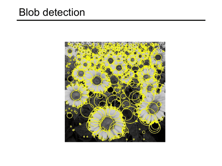
Blob detection
Feature detection with scale selection
•
We want to extract features with characteristic
scale that is covariant with the image
transformation
Blob detection: Basic idea
• To detect blobs, convolve the image with a
“blob filter” at multiple scales and look for
extrema of filter response in the resulting
scale space
Blob detection: Basic idea
minima
*
=
maxima
Find maxima and minima of blob filter response
in space and scale
Source: N. Snavely
Blob filter
Laplacian of Gaussian: Circularly symmetric
operator for blob detection in 2D
 g  g
 g 2  2
x
y
2
2
2
Recall: Edge detection
f
d
g
dx
d
f
g
dx
Edge
Derivative
of Gaussian
Edge = maximum
of derivative
Source: S. Seitz
Edge detection, Take 2
f
Edge
2
Second derivative
of Gaussian
(Laplacian)
d
g
2
dx
d2
f 2g
dx
Edge = zero crossing
of second derivative
Source: S. Seitz
From edges to blobs
• Edge = ripple
• Blob = superposition of two ripples
maximum
Spatial selection: the magnitude of the Laplacian
response will achieve a maximum at the center of
the blob, provided the scale of the Laplacian is
“matched” to the scale of the blob
Scale selection
• We want to find the characteristic scale of the
blob by convolving it with Laplacians at several
scales and looking for the maximum response
• However, Laplacian response decays as scale
increases:
original signal
(radius=8)
increasing σ
Scale normalization
• The response of a derivative of Gaussian
filter to a perfect step edge decreases as σ
increases
1
 2
Scale normalization
• The response of a derivative of Gaussian
filter to a perfect step edge decreases as σ
increases
• To keep response the same (scale-invariant),
must multiply Gaussian derivative by σ
• Laplacian is the second Gaussian derivative,
so it must be multiplied by σ2
Effect of scale normalization
Original signal
Unnormalized Laplacian response
Scale-normalized Laplacian response
maximum
Blob detection in 2D
Laplacian of Gaussian: Circularly symmetric
operator for blob detection in 2D
Scale-normalized:

 g  g
g    2  2 
y 
 x
2
2
norm
2
2
Scale selection
• At what scale does the Laplacian achieve a maximum
response to a binary circle of radius r?
r
image
Laplacian
Scale selection
• At what scale does the Laplacian achieve a maximum
response to a binary circle of radius r?
• To get maximum response, the zeros of the Laplacian
have to be aligned with the circle
• The Laplacian is given by (up to scale):
( x  y  2 ) e
2
2
2
 ( x 2  y 2 ) / 2 2
• Therefore, the maximum response occurs at
  r / 2.
circle
0
r
Laplacian
image
Characteristic scale
• We define the characteristic scale of a blob
as the scale that produces peak of Laplacian
response in the blob center
characteristic scale
T. Lindeberg (1998). "Feature detection with automatic scale selection."
International Journal of Computer Vision 30 (2): pp 77--116.
Scale-space blob detector
1. Convolve image with scale-normalized
Laplacian at several scales
Scale-space blob detector: Example
Scale-space blob detector: Example
Scale-space blob detector
1. Convolve image with scale-normalized
Laplacian at several scales
2. Find maxima of squared Laplacian response
in scale-space
Scale-space blob detector: Example
Efficient implementation
• Approximating the Laplacian with a
difference of Gaussians:
L   2  Gxx ( x, y,  )  G yy ( x, y,  ) 
(Laplacian)
DoG  G ( x, y, k )  G ( x, y,  )
(Difference of Gaussians)
Efficient implementation
David G. Lowe. "Distinctive image features from scale-invariant
keypoints.” IJCV 60 (2), pp. 91-110, 2004.
From feature detection to feature description
•
Scaled and rotated versions of the same
neighborhood will give rise to blobs that are related
by the same transformation
•
What to do if we want to compare the appearance of
these image regions?
•
Normalization: transform these regions into samesize circles
•
Problem: rotational ambiguity
Eliminating rotation ambiguity
•
To assign a unique orientation to circular
image windows:
•
•
Create histogram of local gradient directions in the patch
Assign canonical orientation at peak of smoothed histogram
0
2
SIFT features
• Detected features with characteristic scales
and orientations:
David G. Lowe. "Distinctive image features from scale-invariant
keypoints.” IJCV 60 (2), pp. 91-110, 2004.
From feature detection to feature description
Detection is covariant:
features(transform(image)) = transform(features(image))
Description is invariant:
features(transform(image)) = features(image)
SIFT descriptors
David G. Lowe. "Distinctive image features from scale-invariant
keypoints.” IJCV 60 (2), pp. 91-110, 2004.
Properties of SIFT
Extraordinarily robust detection and description technique
• Can handle changes in viewpoint
– Up to about 60 degree out-of-plane rotation
• Can handle significant changes in illumination
– Sometimes even day vs. night
• Fast and efficient—can run in real time
• Lots of code available
Source: N. Snavely
Affine adaptation
• Affine transformation approximates viewpoint
changes for roughly planar objects and
roughly orthographic cameras
Affine adaptation
Consider the second moment matrix of the window
containing the blob:
 I x2
M   w( x, y ) 
x, y
 I x I y
IxI y 
 0
1  1
R 
R

2 
I y 
 0 2 
direction of the
fastest change
Recall:
u 
[u v] M    const
v 
(max)-1/2
direction of
the slowest
change
(min)-1/2
This ellipse visualizes the “characteristic shape” of the
window
Affine adaptation example
Scale-invariant regions (blobs)
Affine adaptation example
Affine-adapted blobs