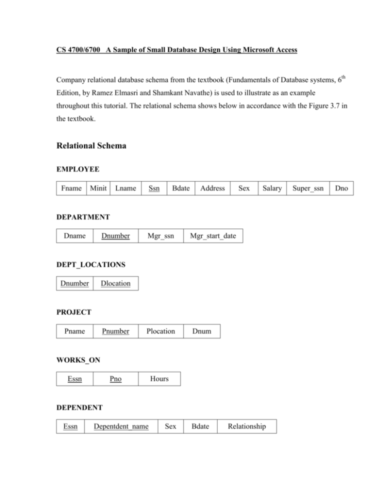
CS 4700/6700 A Sample of Small Database Design Using Microsoft Access
Company relational database schema from the textbook (Fundamentals of Database systems, 6th
Edition, by Ramez Elmasri and Shamkant Navathe) is used to illustrate as an example
throughout this tutorial. The relational schema shows below in accordance with the Figure 3.7 in
the textbook.
Relational Schema
EMPLOYEE
Fname
Minit
Lname
Ssn
Bdate
Address
Sex
Salary
DEPARTMENT
Dname
Dnumber
Mgr_ssn
Mgr_start_date
DEPT_LOCATIONS
Dnumber
Dlocation
PROJECT
Pname
Pnumber
Plocation
Pno
Hours
Dnum
WORKS_ON
Essn
DEPENDENT
Essn
Depentdent_name
Sex
Bdate
Relationship
Super_ssn
Dno
1. Creating a New Database
When you open Microsoft Access 2013 it should look like Figure 1. To create a new database,
you can choose “Blank desktop database”.
Figure 1
Type the name of the database in File Name box of the pop-up window. To save the database at a
different location, click on the highlighted folder symbol. Once the database name is entered
click on the “Create” button. Here the database is named “Company” as shown in Figure 2.
Figure 2
Once the “Create” button is clicked Access will be as shown in Figure 3.
Figure 3
2. Creating New Tables
Click “Create” first, then in the sub tab, click on “Table”. Figure 4 shows how it should appear
when you do the above. Actually, Table 1 is created by default before you creating a new table.
Figure 4
Now under the tab “Home” or tab “Fields”, click on “View” and select “Design View”. Then in
the pop-up window as shown in Figure 5, type the table name and click “OK”. Here,
“EMPLOYEE” is entered as the table name.
Figure 5
Once you click “OK” in previous step, you can start entering the field names or attribute names
and specify the data type from the drop down menu as shown in Figure 6. By default it sets the
first attribute you entered as the primary key. To mark or unmark any of the fields as a primary
key, click on the highlighted primary key symbol.
Figure 6
Note:
To mark two or more attributes as primary keys, first unmark the already existing primary key by
selecting the attribute marked as the primary key and click on the “Primary Key” symbol
highlighted in Figure 7 (optional). Then select the two or more attributes you want to set as
primary keys, for instance, “Dnumber” and “Dlocation” shown in Figure 7. At last, click on the
“Primary Key” symbol.
Figure 7
In the encircled area shown in Figure 8, constrains can be made on the input data of attributes.
For example, in Figure 8, the “Field Size” of “Sex” is set to be 1. And The “Validation Rule” is
set to be “M or F or U” which means that the input of attribute “Sex” can only be “M”, “F” or
“U” for unknown. When the input data are invalid, the message in “Validation Text” will be
popped up to remind users.
Figure 8
After inputting all the field names of a table and their data types, click on “View” and select
“Datasheet View”.
Figure 9
Once you select the “Datasheet View”, the dialogue box shown in Figure 10 pops up, asking if
you want to save the table. Select “Yes”.
Figure 10
Once “Yes” is selected, a datasheet appears as in Figure 11. Here you can start entering data row
by row in the EMPLOYEE table.
Figure 11
Repeat all the steps of “Creating New Tables”, you can create all other tables in your database.
And the completed database looks like Figure 12. Input data comes from the Figure 3.6 in the
textbook.
Figure 12
3. Adding Relationships
Once all the tables of the database are created, we need to specify referential integrity
constraints. To do this, click on “Database Tools” and select “Relationships”.
Figure 13
When “Relationships” is clicked, the “Show Table” window pops up as in Figure 14. Or you can
open the “Show Table” by clicking on the highlighted symbol.
Figure 14
In the “Show Table”, select all tables you want to establish relationships then click the “Add”
button. These tables will appear on the background board as shown in Figure 15. Once you have
finished adding tables, click on the “Close” button to close the “Show Table”.
Figure 15
The referential integrity constraint between two relations can be specified by dragging the
primary key attribute of one table (e.g., “Ssn” in the EMPLOYEE table) to the foreign key
attribute of the other table (e.g., “Essn” in the WORKS_ON table). Then “Edit Relationships”
window appears like Figure 16. Make sure that the relationship is made between appropriate
attributes by checking the attribute and table names in the “Table/Query” and “Related Table
/Query”. Sometime by dragging operations, unrelated attributes may be connected incorrectly, so
always check the attribute names before clicking on “Create”. Once you click on “Create”, a line
connecting these two attributes will appear as shown in Figure 17.
Figure 16
Figure 17
Repeat the same procedures in adding relationships to other tables in the database. Figure 18
presents the final result when all the relationships have been established. Note that if a
relationship is needed between attributes in the same table, a copy of the table should be
generated like table “EMPLOYEE_1” in Figure 18. Moreover when there is more than one
relationship between two tables, like “EMPLOYEE” and “DEPARTMENT”, then a copy of one
of the table is also need to be created. And the copy table is still “EMPLOYEE_1” in this more
than one relationship situation.
Figure 18
To exit from “Relationship Tools”, click on any of the encircled areas in Figure 19. A dialogue
box asking “Do you want to save changes to the layout of ‘relationships’” appears. Click on
‘Yes’.
Figure 19
4. Writing Queries
To start writing queries, click on “Create” then “Query Design”.
Figure 20
Click on ‘Close’ to close the pop-up ‘Show Table’ window.
Figure 21
Now click on “SQL View” then select “SQL SQL View”.
Figure 22
Once ‘SQL SQL View’ is selected, Figure 23 appears. SQL queries can be written on the
provided space as shown below. To run the query, click the “! run” button.
Figure 23
Some sample queries is used as illustrations.
Query 1: Retrieve the name and address of all employees who work for the ‘Research’
Department.
Figure 24
After running the query, the result will show on the screen as in Figure 25.
Figure 25
Query 2: Retrieve the name of each employee who works on all the projects controlled by
department 4.
Figure 26
Result of this query is shown in Figure 27.
Figure 27
Query 3: For each project, retrieve the project number, the project name and the number of
employees who work on that project.
Figure 28
Result of this query is shown as:
Figure 29