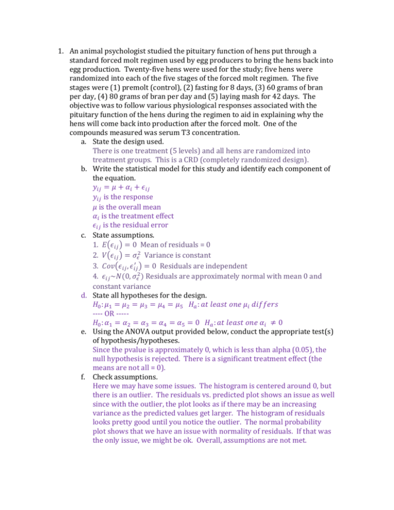
1. An animal psychologist studied the pituitary function of hens put through a
standard forced molt regimen used by egg producers to bring the hens back into
egg production. Twenty-five hens were used for the study; five hens were
randomized into each of the five stages of the forced molt regimen. The five
stages were (1) premolt (control), (2) fasting for 8 days, (3) 60 grams of bran
per day, (4) 80 grams of bran per day and (5) laying mash for 42 days. The
objective was to follow various physiological responses associated with the
pituitary function of the hens during the regimen to aid in explaining why the
hens will come back into production after the forced molt. One of the
compounds measured was serum T3 concentration.
a. State the design used.
There is one treatment (5 levels) and all hens are randomized into
treatment groups. This is a CRD (completely randomized design).
b. Write the statistical model for this study and identify each component of
the equation.
𝑦𝑖𝑗 = 𝜇 + 𝛼𝑖 + 𝜖𝑖𝑗
𝑦𝑖𝑗 is the response
𝜇 is the overall mean
𝛼𝑖 is the treatment effect
𝜖𝑖𝑗 is the residual error
c. State assumptions.
1. 𝐸(𝜖𝑖𝑗 ) = 0 Mean of residuals = 0
2. 𝑉(𝜖𝑖𝑗 ) = 𝜎𝜖2 Variance is constant
′
3. 𝐶𝑜𝑣(𝜖𝑖𝑗 , 𝜖𝑖𝑗
) = 0 Residuals are independent
2
4. 𝜖𝑖𝑗 ~𝑁(0, 𝜎𝜖 ) Residuals are approximately normal with mean 0 and
constant variance
d. State all hypotheses for the design.
𝐻0 : 𝜇1 = 𝜇2 = 𝜇3 = 𝜇4 = 𝜇5 𝐻𝑎 : 𝑎𝑡 𝑙𝑒𝑎𝑠𝑡 𝑜𝑛𝑒 𝜇𝑖 𝑑𝑖𝑓𝑓𝑒𝑟𝑠
---- OR ----𝐻0 : 𝛼1 = 𝛼2 = 𝛼3 = 𝛼4 = 𝛼5 = 0 𝐻𝑎 : 𝑎𝑡 𝑙𝑒𝑎𝑠𝑡 𝑜𝑛𝑒 𝛼𝑖 ≠ 0
e. Using the ANOVA output provided below, conduct the appropriate test(s)
of hypothesis/hypotheses.
Since the pvalue is approximately 0, which is less than alpha (0.05), the
null hypothesis is rejected. There is a significant treatment effect (the
means are not all = 0).
f. Check assumptions.
Here we may have some issues. The histogram is centered around 0, but
there is an outlier. The residuals vs. predicted plot shows an issue as well
since with the outlier, the plot looks as if there may be an increasing
variance as the predicted values get larger. The histogram of residuals
looks pretty good until you notice the outlier. The normal probability
plot shows that we have an issue with normality of residuals. If that was
the only issue, we might be ok. Overall, assumptions are not met.
Normal Q-Q Plot
0
-4
-3
-2
-1
0
1
2
-4
-2
0
2
4
Residuals vs. Predicted
100
120
140
hens.pred
-1
-2
-1
0
Theoretical Quantiles
hens.resid
hens.resid
-2
-4
-3
2
4
Frequency
6
Sample Quantiles
0
8
1
10
Histogram of hens.resid
160
180
1
2
2. The self-inductance of coils with iron-oxide cores was measured under different
temperature conditions of the measuring bridge. The coil temperature was held
constant. Five coils were used for the experiment. The self-inductance of each
coil was measured for each of the four temperatures (22°, 23°, 24° and 25°) for
the measuring bridge. The temperatures were utilized in a random order for
each coil. The measured response was percentage deviations from a standard.
a. State the design used.
Each coil is considered a block since each one was measured at each of
the four temperatures. This is a Randomized Complete Block Design
(RCBD).
b. Write the statistical model for this study and identify each component of
the equation.
𝑦𝑖𝑗 = 𝜇 + 𝛼𝑖 + 𝛽𝑗 + 𝜖𝑖𝑗
𝑦𝑖𝑗 is the response
𝜇 is the overall mean
𝛼𝑖 is the treatment effect
𝛽𝑗 is the block effect
𝜖𝑖𝑗 is the residual error
c. State all hypotheses for the design.
𝐻0 : 𝛼1 = 𝛼2 = 𝛼3 = 𝛼4 = 0 𝐻𝑎 : 𝑎𝑡 𝑙𝑒𝑎𝑠𝑡 𝑜𝑛𝑒 𝛼𝑖 ≠ 0
d. Using the ANOVA output provided below, conduct the appropriate test(s)
of hypothesis/hypotheses.
Since we only need to check the F statistic for the treatment (here it’s the
temperature), the pvalue is 0.005319 which is smaller than alpha (0.05)
so the null hypothesis would be rejected. The treatment effect is
significant.
e. Check assumptions.
The histogram of residuals is mostly centered around 0. The residuals vs.
predicted plot shows no increasing or decreasing variance (so it’s
constant). However, the normality assumption may have been violated.
The histogram of residuals is symmetric but there are some outliers. The
normal probability plot shows that there are four possible outliers
(meaning that normality is not happening). Assumptions may be met, but
the normality of residuals is not.
Residuals vs. Predicted
0.00
coil.resid
-0.02
0.00
-0.04
-0.04
-0.02
Sample Quantiles
0.02
0.02
0.04
0.04
Normal Q-Q Plot
-2
-1
0
1
2
0
1
2
Frequency
3
4
5
Histogram of coil.resid
-0.04
-0.02
0.00
coil.resid
0.2
0.4
0.6
0.8
coil.pred
Theoretical Quantiles
0.02
0.04
1.0
1.2
1.4
3. A traffic engineer conducted a study to compare the total unused red light time
for five different traffic light signal sequences. The experiment was conducted
over five intersections and five time periods.
a. State the design used.
The intersection and the time period are both blocks with the light
sequence being the treatment where every “row” and “column” have each
level of the treatment. This is a Latin Squares Design.
b. Write the statistical model for this study and identify each component of
the equation.
𝑦𝑖𝑗𝑘 = 𝜇 + 𝛼𝑖 + 𝛽𝑗 + 𝛾𝑘 + 𝜖𝑖𝑗𝑘
𝑦𝑖𝑗𝑘 is the response
𝜇 is the overall mean
𝛼𝑖 is the treatment effect
𝛽𝑗 is the block 1 effect (rows)
𝛾𝑘 is the block 2 effect (columns)
𝜖𝑖𝑗𝑘 is the residual error
c. State all hypotheses for the design.
𝐻0 : 𝛼1 = 𝛼2 = 𝛼3 = 𝛼4 = 𝛼5 𝐻𝑎 : 𝑎𝑡 𝑙𝑒𝑎𝑠𝑡 𝑜𝑛𝑒 𝛼𝑖 ≠ 0
d. Using the ANOVA output provided below, conduct the appropriate test(s)
of hypothesis/hypotheses.
The only test we do here is for the treatment since the other two are
blocks. The pvalue for treatment is 0.04976, and is less than alpha (0.05).
While it’s close, we will still reject the null hypothesis. The treatment
effect (the timing sequence) is significant (marginally, but still
significant).
e. Check assumptions.
The histogram of residuals is centered around 0. The residuals vs.
predicted values plot looks random so the variance of the residuals is
constant. The histogram of residuals is not quite symmetric, but is
probably approximately normal enough to say that the residuals have a
normal distribution (there’s no outliers so it should be ok).
Residuals vs. Predicted
1
-1
-2
-3
-2
-3
-2
-1
0
1
15
2
0
2
4
6
8
Histogram of traffic.resid
-3
-2
-1
0
1
traffic.resid
20
25
traffic.pred
Theoretical Quantiles
Frequency
0
traffic.resid
1
0
-1
Sample Quantiles
2
2
3
3
Normal Q-Q Plot
2
3
4
30
4. A chemical production process consists of a first reaction with an alcohol and a
section reaction with a base. In this experiment, the alcohol has three levels and
the base has two. The data collected were the percent yield.
a. State the design used.
Here we have two treatments, one with 3 levels and one with 2 levels.
This is a 3X2 factorial design (completely randomized factorial design –
CRF).
b. Write the statistical model for this study and identify each component of
the equation.
𝑦𝑖𝑗𝑘 = 𝜇 + 𝛼𝑖 + 𝛽𝑗 + 𝛾𝑘 + 𝜖𝑖𝑗𝑘 OR 𝑦𝑖𝑗𝑘 = 𝜇 + 𝛼𝑖 + 𝛽𝑗 + (𝛼𝛽)𝑖𝑗 + 𝜖𝑖𝑗𝑘
𝑦𝑖𝑗𝑘 is the response
𝜇 is the overall mean
𝛼𝑖 is the treatment A effect
𝛽𝑗 is the treatment B effect
𝛾𝑘 𝑜𝑟 (𝛼𝛽)𝑖𝑗 is the interaction between treatments A and B.
𝜖𝑖𝑗𝑘 is the residual error
c. State all hypotheses for the design.
Main effects:
A 𝐻0 : 𝛼1 = 𝛼2 = 𝛼3 = 0 𝐻𝑎 : 𝑎𝑡 𝑙𝑒𝑎𝑠𝑡 𝑜𝑛𝑒 𝛼𝑖 ≠ 0
B 𝐻0 : 𝛽1 = 𝛽2 = 0 𝐻𝑎 : 𝑎𝑡 𝑙𝑒𝑎𝑠𝑡 𝑜𝑛𝑒 𝛽𝑗 ≠ 0
Interaction: (use either alpha-beta or gamma symbols)
AB 𝐻0 : 𝛼1 𝛽1 = 𝛼2 𝛽2 = 𝛼3 𝛽3 = 𝛼4 𝛽4 = 𝛼5 𝛽5 = 𝛼6 𝛽6 = 0
𝐻𝑎 : 𝑎𝑡 𝑙𝑒𝑎𝑠𝑡 𝑜𝑛𝑒 𝛼𝛽𝑖𝑗 ≠ 0
d. Using the ANOVA output provided below, conduct the appropriate test(s)
of hypothesis/hypotheses.
Main effects:
A: the pvalue is 0.29149, which is greater than alpha so we would not
reject the null for treatment A effects being significant (A is not
significant)
B: the pvalue is 0.09103 which is greater than alpha so we would not
reject the null for treatment B effects being significant (B is not
significant)
Interaction:
AB: the pvalue is 0.01346 which is less than alpha so we reject the null
hypothesis. That means the interaction between the treatments is
significant.
e. Check assumptions.
The histogram of the residuals looks to be centered on 0. The residual vs.
predicted plot looks to be random scatter so the variance is constant. The
histogram of residuals looks a bit right skewed (and it showed on the
normal probability plot) but the skew shouldn’t be too bad. So, the
residuals are approximately normal.
Residuals vs. Predicted
-2
-1
0
1
2
0
1
2
3
4
5
6
7
Histogram of chem.resid
-2
-1
0
1
chem.resid
89.0
89.5
90.0
90.5
chem.pred
Theoretical Quantiles
Frequency
0
chem.resid
-1
0
-1
Sample Quantiles
1
1
2
2
Normal Q-Q Plot
2
3
91.0
91.5
92.0
5. A field plot experiment was conducted to evaluate the interaction between
timing of nitrogen application to the soil (early, optimum, late) and two levels of
a nitrification inhibitor (none, 0.5 lb/acre), all on three separate plots of the field.
The inhibitor delays conversion of ammonium forms of nitrogen into a more
mobile nitrate form to reduce leaching losses of fertilizer-derived nitrates. The
nitrogen was supplied as pulse-labeled 15N through a drip irrigation system at an
early, an optimum, and a late date of application. The data are the percent 15N
taken up by sweet corn plants grown on the three plots.
a. State the design used.
We have three different plots that are to be used as blocks (since there
could be variation in plants due to different soils in each plot), two
different treatments (inhibitor and timing). This is a factorial treatment
structure in a randomized block design (FDRB).
b. Write the statistical model for this study and identify each component of
the equation.
𝑦𝑖𝑗𝑘 = 𝜇 + 𝛼𝑖 + 𝛽𝑗 + 𝛾𝑘 + (𝛼𝛾)𝑖𝑘 + 𝜖𝑖𝑗𝑘
𝑦𝑖𝑗𝑘 is the response
𝜇 is the overall mean
𝛽𝑗 is the block effect
𝛼𝑖 is treatment A effect (timing)
𝛾𝑘 is treatment B effect (inhibitor)
(𝛼𝛾)𝑖𝑘 is the interaction between treatments A and B.
𝜖𝑖𝑗𝑘 is the residual error
c. State all hypotheses for the design.
Main effects:
A 𝐻0 : 𝛼1 = 𝛼2 = 𝛼3 = 0 𝐻𝑎 : 𝑎𝑡 𝑙𝑒𝑎𝑠𝑡 𝑜𝑛𝑒 𝛼𝑖 ≠ 0
B 𝐻0 : 𝛾1 = 𝛾2 = 0 𝐻𝑎 : 𝑎𝑡 𝑙𝑒𝑎𝑠𝑡 𝑜𝑛𝑒 𝛾𝑘 ≠ 0
Interaction:
AB 𝐻0 : 𝛼1 𝛾1 = 𝛼2 𝛾2 = ⋯ = 𝛼12 𝛾12 = 0
𝐻𝑎 : 𝑎𝑡 𝑙𝑒𝑎𝑠𝑡 𝑜𝑛𝑒 𝛼𝛾𝑖𝑘 ≠ 0
d. Using the ANOVA output provided below, conduct the appropriate test(s)
of hypothesis/hypotheses.
Main effects:
A: the pvalue is 0.005, which is less than alpha so we would reject the
null for treatment A effects being significant (A is significant)
B: the pvalue is 0.005 which is less than alpha so we would reject the null
for treatment B effects being significant (B is significant)
Interaction:
AB: the pvalue is 0.08669 which is greater than alpha so we do not reject
the null hypothesis. That means the interaction between the treatments
is not significant.
e. Check assumptions.
The histogram of the residuals looks to be centered on 0. The residual vs.
predicted plot looks to be random scatter so the variance is constant. The
histogram of residuals looks a bit left skewed (and it showed on the
normal probability plot) but the skew shouldn’t be too bad. So, the
residuals are approximately normal.
Normal Q-Q Plot
-5
0
corn.resid
5
0
-5
-15
-10
-10
Sample Quantiles
10
5
15
Residuals vs. Predicted
-2
-1
0
Theoretical Quantiles
1
2
20
30
40
corn.pred
50
60
3
2
1
0
Frequency
4
5
6
Histogram of corn.resid
-15
-10
-5
0
corn.resid
5
10