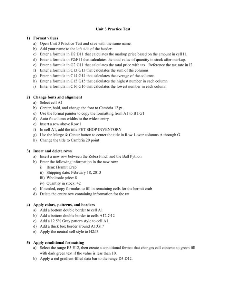
Unit 3 Practice Test
1) Format values
a) Open Unit 3 Practice Test and save with the same name.
b) Add your name to the left side of the header.
c) Enter a formula in D2:D11 that calculates the markup price based on the amount in cell I1.
d) Enter a formula in F2:F11 that calculates the total value of quantity in stock after markup.
e) Enter a formula in G2:G11 that calculates the total price with tax. Reference the tax rate in I2.
f) Enter a formula in C13:G13 that calculates the sum of the columns
g) Enter a formula in C14:G14 that calculates the average of the columns
h) Enter a formula in C15:G15 that calculates the highest number in each column
i) Enter a formula in C16:G16 that calculates the lowest number in each column
2) Change fonts and alignment
a) Select cell A1
b) Center, bold, and change the font to Cambria 12 pt.
c) Use the format painter to copy the formatting from A1 to B1:G1
d) Auto fit column widths to the widest entry
e) Insert a row above Row 1
f) In cell A1, add the title PET SHOP INVENTORY
g) Use the Merge & Center button to center the title in Row 1 over columns A through G.
h) Change the title to Cambria 20 point
3) Insert and delete rows
a) Insert a new row between the Zebra Finch and the Ball Python
b) Enter the following information in the new row:
i) Item: Hermit Crab
ii) Shipping date: February 18, 2013
iii) Wholesale price: 8
iv) Quantity in stock: 42
c) If needed, copy formulas to fill in remaining cells for the hermit crab
d) Delete the entire row containing information for the rat
4) Apply colors, patterns, and borders
a) Add a bottom double border to cell A1
b) Add a bottom double border to cells A12:G12
c) Add a 12.5% Gray pattern style to cell A1.
d) Add a thick box border around A1:G17
e) Apply the neutral cell style to H2:I3
5) Apply conditional formatting
a) Select the range E3:E12, then create a conditional format that changes cell contents to green fill
with dark green text if the value is less than 10.
b) Apply a red gradient-filled data bar to the range D3:D12.
6) Apply cell formats
a) Apply month/day/year formatting to the dates in column B. Auto fit the column width.
b) Apply accounting formatting with two decimal places to C3:D3
c) Apply comma formatting with two decimal places to C4:D12
d) Apply accounting formatting with two decimal places to all remaining monetary amounts
e) Apply % formatting with two decimal places to I2 and I3
7) Rename and move a worksheet
a) Name the Sheet 1 tab Current Inventory
b) Name the Sheet 3 tab Future Inventory
c) Change the Current Inventory tab color to blue
d) Change the Future Inventory tab color to green
e) Move the Future Inventory tab so it comes after (to the right of) the Current Inventory tab
8) Check spelling and print
a) Check the spelling in the worksheet using the spell checker, and replace any spelling errors if
necessary.
b) Change page orientation to landscape
c) Scale the worksheet so all columns print on one page
d) Save your changes and print one sheet with formulas and a second sheet without formulas. Staple
both pages together.
e) Compare your worksheet to the answer key