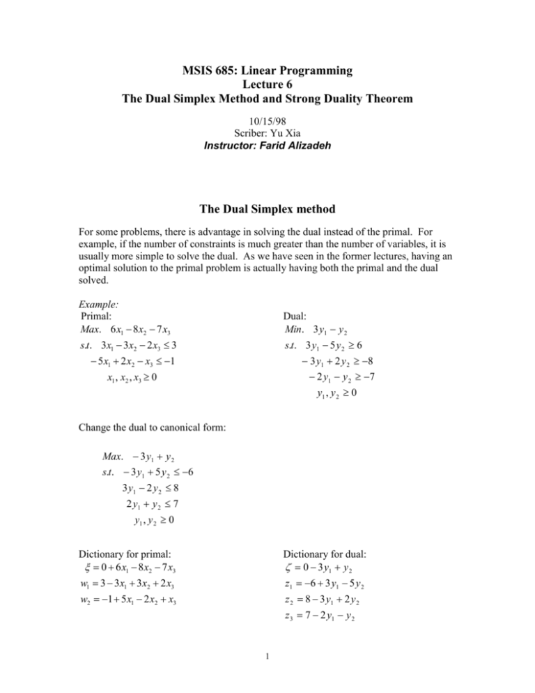
MSIS 685: Linear Programming
Lecture 6
The Dual Simplex Method and Strong Duality Theorem
10/15/98
Scriber: Yu Xia
Instructor: Farid Alizadeh
The Dual Simplex method
For some problems, there is advantage in solving the dual instead of the primal. For
example, if the number of constraints is much greater than the number of variables, it is
usually more simple to solve the dual. As we have seen in the former lectures, having an
optimal solution to the primal problem is actually having both the primal and the dual
solved.
Example:
Primal:
Max. 6 x1  8 x2  7 x3
Dual:
Min. 3 y1  y 2
s.t. 3 x1  3x2  2 x3  3
s.t. 3 y1  5 y 2  6
 3 y1  2 y 2  8
 5 x1  2 x2  x3  1
 2 y1  y 2  7
x1 , x2 , x3  0
y1 , y 2  0
Change the dual to canonical form:
Max.  3 y1  y 2
s.t.  3 y1  5 y 2  6
3 y1  2 y 2  8
2 y1  y 2  7
y1 , y 2  0
Dictionary for primal:
  0  6 x1  8 x2  7 x3
Dictionary for dual:
  0  3 y1  y 2
w1  3  3 x1  3 x2  2 x3
z1  6  3 y1  5 y 2
w2  1  5 x1  2 x2  x3
z 2  8  3 y1  2 y 2
z 3  7  2 y1  y 2
1
Corresponding data matrix:
6  8  7
0

2 
TP   3  3 3
 1 5  2 1 
 0 3 1 
  6 3  5

TD  
 8 3 2 


 7  2  1
Answer:
The optimal dictionary of the primal:
  6  2 x 2  11x3  2w1
x1  1  x 2  2 3 x3  13 w1
w2  4  3x 2  7 3 x3  5 3 w1
Data matrix of the primal optimal solution:
6  2  11  2
2
1 
T  1 1
3
3

7

5
3
3
4 3

*
P
Data matrix of the dual optimal solution:
  6  1  4
 2  1  3
*

TD  
 11  2 3 7 3 


5
1
3
3 
2
Dual optimal dictionary:
  6  z1  4 y2
z 2  2  z1  3 y2
z3  11  3 2 z1  7 3 y2
y1  2  13 z1  5 3 y2
Both the primal and the dual can always be adjusted into canonical form.
From the relation between the dual and the primal we get: TD  TPT
 G (not singular), TP*  GTP  TP*T  TPT G T  TPT  TP*T
TP* is the data matrix represents the optimal dictionary, so its first row except the first
element are not greater than 0, its first column except the first element are not less than 0.
So  TP*T is the corresponding data matrix of an optimal dictionary of the dual.
2
Through the dual simplex method, we move from one dictionary to another while
maintaining the optimality conditions, and terminate when the feasibility conditions are
satisfied. Through the primal simplex method, however, the feasibility conditions are
maintained and we try to reach the optimality conditions.
Usually, after a new constraint is introduced, the former optimal solution will not be
feasible. In this situation, there is often advantage in applying dual simplex method to
the data matrix produced by adding the old optimal data matrix with a new row and
sometimes a new column contributed by the new constraint.
Example 1:
Add a new constraint to the above primal LP problem: x1  1 2
Max. 6 x1  8 x 2  7 x3
s.t. 3x1  3x 2  2 x3  3
 5 x1  2 x 2  x3  1
x1 
1
2
x1 , x 2 , x3  0
Correspondingly, add w3  1 2  x1  1 2  x2  2 3 x3  13 w1 to the basic solution:
  6  2 x2  11x3  2w1
x1  1  x2  2 3 x3  13 w1
w2  4  3x2  7 3 x3  5 3 w1
w3  1 2  x2  2 3 x3  13 w1
The corresponding dual dictionary satisfies feasibility conditions, but not the optimal
conditions. So we can solve the dual instead. Below, we use dual simplex method.
For the primal dictionary, in order to satisfiy feasibility conditions, w3 must leave, and
since w1 is the only variable having positive coefficient in that equation, w1 must enter:
  3  8 x 2  15 x3  6w3
x1 
1
2
 1 3 w3
w2  3 2  2 x 2  x3  5w3
w1  3 2  3x2  2 x3  3w3
We get the optimal solution to the new problem with only one more step.
If there exists an equation, its constant is negative and none of the coefficients are
positive, then the problem is not feasible.
3
Example 2:
  4  x1  2 x2  3x3
x 4  1  3x1  2 x 2  2 x3
x5  2  x1  x 2  2 x3
x6  1  2 x1  2 x 2  2 x3
First choose leaving variable xi , i  arg max  bi : bi  0 , then choose entering variable
xk .
Plug x k  
bi
aik

  (c0  bi a c k ) 
ik

aij
aik
j i ,k
 (c
j i ,k
j

xj  1
aij
aik
aik
xi into  :
c k ) x j  (c i  1
aik
c k ) xi
In order to maintain optimality:
a
c
 c

c
c j  ij ck  0  j  k
(a  0)  k  arg min  j : aij  0
aik
aij
aik ij
a
ij


In this example, we choose x5 to leave and x3 to enter the base. Of cause x 2 may leave
if another rule is applied.
One application of dual simplex method is in integer programming. One of the algorithm
for integer programming is first solving the problem without the integrity constraints,
then imposing the constraints one by one. For example, consider the following problem:
Max c T X
s.t. AX  b
X 0
X : Integers
First get the optimal solution to its LP relaxation:
Max c T X
s.t. AX  b .
X 0
If we get x17  49.7 , then we divide the LP relaxation into two parts by adding extra
constrains:
4
Max c T X
s.t. AX  b
X 0
x17  50
Max c T X
s.t. AX  b
X 0
x17  49
The branching goes on through adding further constraints.
Strong Duality Theorem
Separation Theorem1:
If Cn is closed and convex, and if x0C, then there exits a hyper-plane separating x0
and C, i.e. H: wT x  b , such that
wT x 0  b
wT z  b
 z  C 
Intuition interpretation:
wT x  b
C
.
x0
The constraints that C is convex and closed are necessary:
If C is not convex:
C
.
x0
If C is not closed:
5
C (a circle without point x0)
x0
Proof skeleton:
C is closed, so  z 0  C , s.t. x0  z 0  inf  x0  z : z  C  0
Draw a hyper-plane wT x  b between x0 and z 0 , not through x0 , and perpendicular to
line x0 z 0 . So
wT x 0  b
wT z  b
 z  C 
Separation Theorem2:
If C1 , C2  n, closed and convex, then if C1  C2   , there exits a seperating hyperplane H: wT x  b between C1 and C2 , s.t. z  C1 , wT z  b ; v  C2 , wT v  b
Proof:
 z 0  C1 , v0  C 2 , such that z0  v0  inf  z  v : z  C1 , v  C2   0 .
Use the same method as that to prove separation therorem1.
Cone:
Definition: A subset K n is a cone if x  K  x  K (  0)
A cone is pointed if K  K  0 .
A cone K is convex, iff x, y  K , x  y  K .
Proof:
: K is convex  1 2 x  1 2 y  K  2( 1 2 x  1 2 y)  K
: K is a cone  x  K , (1   ) y  K  x  (1   ) y  K
Separating Hyper-plane Theorem for Cones:
If K is a closed convex cone, and x0 K, then there exists a linear space separating x0 and
K; i.e.  wT x  0 , s.t. wT x0  0 , wT z  0
 z  K  .
6
Farka’s Lemma: 1
For any matrix A  m*n and vector b  m, either x  n , x  0 , Ax  b or  y m,
AT y  0 , b T y  0 , but not both.
Proof: Let K= x1a1    xn an : xi  0, so K is a closed convex cone.
If b  K, then  x  0 , Ax  b ; otherwise, according to separating hyper-plane theorem
for cones,  y, such that y T b  0 , y T ai  0 i  1,n .
Proof of Strong Duality Theorem Based on Farka’s Lemma:
Strong Duality Theorem: 2
Min. c T X
Max b T y
(D)
(P)
s.t. AX  b
s.t. AT y  c
X 0
If both (P) and (D) are feasible and bounded, then  optimal solution x * to (P) and
optimal solution y * to (D), c T x *  b T y * .
Proof: use contradition:
If the theorem is false, then there exist optimal solution x * to (P) and optimal solution
y * to (D), such that c T x *  b T y *  z 0 . That means the following problem is not feasible:
b
 A
c T  x   z  ( x  0) .
 
 0
T
T
y
b  y 
 A  y 
Use Farkas lemma,   , s.t.  T     0,      0 .
c   y 0 
 y0 
 z0   y0 
Namely: b T y  z 0 y 0  0 (1)
AT y  y 0 c  0 (2)
Case 1: y 0  0
Divide both sides of (1) and (2) by  y 0 
  z , AT  y

bT  y

  y   c . It is contradictory to z 0 is the optimum to (D).
0
0
  y0 

Case 2: y0  0
So (1) and (2) equal to b T y  0 , AT y  0 . According to Farkas lemma, Ax  b ( x  0) is
not feasible.
In the textbook, LP simplex method is first given; from it, duality theory is proved; then Farka’s lemma is
proved; and then convex analysis and a lot of other stuff are given.
In this lecture, we start from the separating theorem; then use it to prove Farka’s lemma; then use Farka’s
lemma to prove duality in LP; and we can also get a lot of other results.
1
2
c T x  ( AT y) T x  y T b . Through contradiction, it is easy to prove that if (P) is unbounded, then (D) is
not feasible; if (D) is unbounded, then (P) is not feasible.
7
Case 3: y 0  0
Divide both sides of (1) and (2) by  y 0  :

b T  y   z 0  0
y
0


 (3)
T y

A 
  c  0 
 y0 

T *
b y z

Add T * 0  to (3):
A y  c  0

b T  y  y *   0 
y
0




T y
*
A 
 y   0

 y0

According to Farkas' lemma, there is no solution to Ax  b ( x  0) .
8