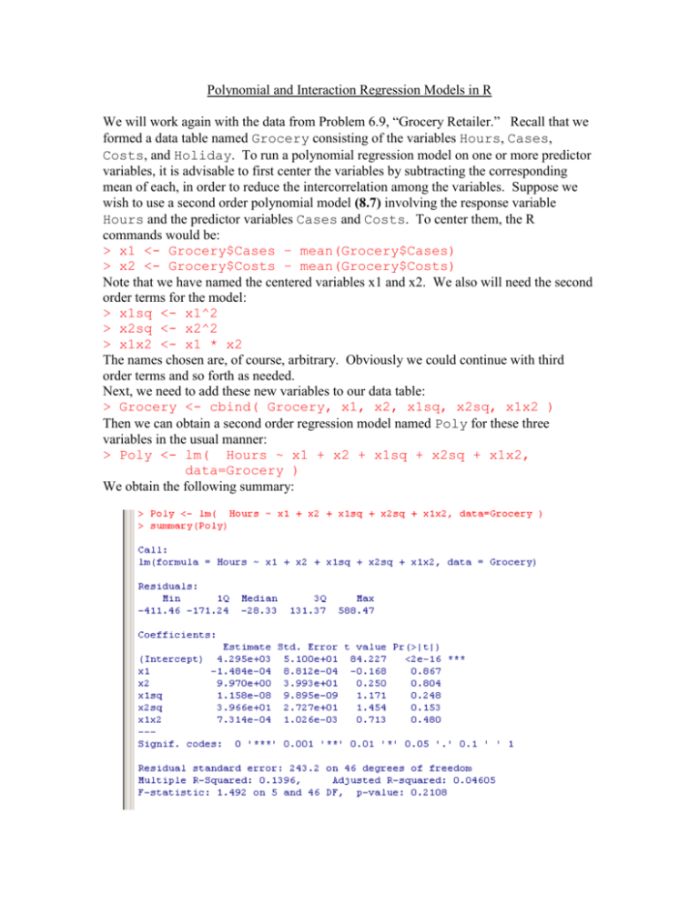
Polynomial and Interaction Regression Models in R
We will work again with the data from Problem 6.9, “Grocery Retailer.” Recall that we
formed a data table named Grocery consisting of the variables Hours, Cases,
Costs, and Holiday. To run a polynomial regression model on one or more predictor
variables, it is advisable to first center the variables by subtracting the corresponding
mean of each, in order to reduce the intercorrelation among the variables. Suppose we
wish to use a second order polynomial model (8.7) involving the response variable
Hours and the predictor variables Cases and Costs. To center them, the R
commands would be:
> x1 <- Grocery$Cases – mean(Grocery$Cases)
> x2 <- Grocery$Costs – mean(Grocery$Costs)
Note that we have named the centered variables x1 and x2. We also will need the second
order terms for the model:
> x1sq <- x1^2
> x2sq <- x2^2
> x1x2 <- x1 * x2
The names chosen are, of course, arbitrary. Obviously we could continue with third
order terms and so forth as needed.
Next, we need to add these new variables to our data table:
> Grocery <- cbind( Grocery, x1, x2, x1sq, x2sq, x1x2 )
Then we can obtain a second order regression model named Poly for these three
variables in the usual manner:
> Poly <- lm( Hours ~ x1 + x2 + x1sq + x2sq + x1x2,
data=Grocery )
We obtain the following summary:
Note that the P-values for the t-tests for the parameter estimates corresponding to each
predictor are each greater than 0.10, and so is the P-value for the F-test, which tells us
that all the predictors can be dropped from the model. Clearly, this model is not
appropriate.
Let's try a second-order polynomial regression model (8.1) involving only one centered
predictor, x2, associated with the variable Costs. We'll call it Poly2:
> Poly2 <- lm( Hours ~ x2 + x2sq, data=Grocery )
We get the following summary:
Again, the P-values are large for the t-tests and the F-test, indicating that both predictors
can be dropped. Hence this model is not appropriate either.
The estimated regression function, based on a least squares fit, is
Yˆ  4333.44  25.97 x2  39.21x22
Although this model is not valid, let's see how to plot the estimated regression function.
First plot the response variable against the centered predictor x2 in the usual manner:
> plot( Grocery$x2, Grocery$Hours, main="Polynomial Model",
xlab="Costs(centered)", ylab="Hours", pch=19 )
We get the following scatterplot:
4400
4000
Hours
4800
Polynomial Model
-2
-1
0
1
2
Costs(centered)
Now to superimpose the estimated regression function, we first form a vector that
encompasses the range of the horizontal axis, incremented by a suitably small value. It
appears that the horizontal axis ranges between -3 and 3, so we will use an increment
value of 0.1 to form the vector:
> vec <- seq(-3, 3, by=0.1)
We then use the lines() function to superimpose the regression curve, which is obtained
by inputting the vector into the estimated regression function:
> lines( vec, 4333.24 + 25.97*vec + 39.21*vec^2 )
We then have the following plot of the data with the fitted regression function:
4600
4400
4200
4000
Hours
4800
5000
Polynomial Model
-2
-1
0
Costs(centered)
1
2
This is the best second-degree polynomial fit to the data, yet it is obviously not an
appropriate model, as confirmed by the summary table.
We can also run an interaction model (8.29) involving all three of our predictor variables
and the same response variable. We will need to also center the third predictor,
Holiday, and add that centered variable to the data table:
> x3 <- Grocery$Holiday – mean(Grocery$Holiday)
> Grocery <- cbind( Grocery, x3 )
We will then run an interaction model, call it Interact, involving all three centered
variables and the response variable Hours:
> Interact <- lm( Hours ~ x1 + x2 + x3 + x1*x2 + x1*x3 + x2*x3,
data=Grocery )
Note that the interaction terms are indicated in the formula by the asterisk between
variables. We then get the following summary:
By inspecting the P-values for the individual t-tests, it appears that the only terms that
should be kept in the model are x3, corresponding to Holiday, and maybe x1, depending
on the level of significance desired. So an interaction model does not fit the data well at
all.
Whether or not the model is a good fit, we can conduct all the various hypothesis tests,
obtain all the various confidence intervals, and perform all the diagnostics that have been
discussed in previous chapters, using the same techniques. However, to obtain a
confidence interval for the mean response at some vector Xh, we have to make sure we
first center Xh, since our model is based on centered predictors. For example, suppose we
are using the second-order polynomial model above, with the single predictor Costs,
and suppose we are interested in a 95% confidence interval for the mean for the response
Hours when Costs = 7.00. Because our model consists of an intercept, a first-degree
term, and a second-degree term, our vector Xh will consist of three elements: a one (for
the intercept), the centered version of Costs = 7.00, and the centered version of Costs
= 7.00 squared. That is,
> X <- c( 1, 7.00 – mean(Grocery$Costs), ( 7.00 –
mean(Grocery$Costs) )^2 )
Then you may proceed as described in the "Multiple Regression in R" handout.