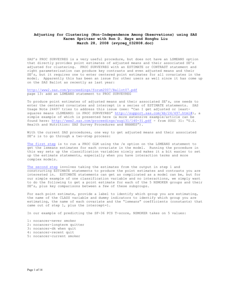
Adjusting for Clustering (Non-Independence Among Observations) using SAS
Karen Spritzer with Ron D. Hays and Honghu Liu
March 28, 2008 (svyreg_032808.doc)
SAS’s PROC SURVEYREG is a very useful procedure, but does not have an LSMEANS option
that directly provides point estimates of adjusted means and their associated SE’s
adjusted for clustering. PROC SURVEYREG with an ESTIMATE or CONTRAST statement and
right parameterization can produce key contrasts and even adjusted means and their
SE’s, but it requires one to enter centered point estimates for all covariates in the
model. Apparently this has been an issue for other users as well since it has come up
on the SAS Ballot as recently as last year:
http://www2.sas.com/proceedings/forum2007/Ballot07.pdf
page 13: add an LSMEANS statement to PROC SURVEYREG
To produce point estimates of adjusted means and their associated SE’s, one needs to
enter the centered covariates and intercept in a series of ESTIMATE statements. SAS
Usage Note 24497 tries to address this issue (see: “Can I get adjusted or leastsquares means (LSMEANS) in PROC SURVEYREG” http://support.sas.com/kb/24/497.html#), a
simple example of which is presented here (a more extensive example/article can be
found here: http://www2.sas.com/proceedings/sugi31/140-31.pdf - from SUGI 31: “U.S.
Health and Nutrition: SAS Survey Procedures and NHANES”).
With the current SAS procedures, one way to get adjusted means and their associated
SE’s is to go through a two-step process:
The first step is to run a PROC GLM using the /e option on the LSMEANS statement to
get the lsmeans estimates for each covariate in the model. Running the procedure in
this way sets up the classification variables nicely and makes it a bit easier to set
up the estimate statements, especially when you have interaction terms and more
complex models.
The second step involves taking the estimates from the output in step 1 and
constructing ESTIMATE statements to produce the point estimates and contrasts you are
interested in. ESTIMATE statements can get as complicated as a model can be, but for
our simple example of one classification variable and no interactions, we simply want
to do the following to get a point estimate for each of the 5 NSMOKER groups and their
SE’s, plus key comparisons between a few of these subgroups.
For each point estimate, provide a label to identify which group you are estimating,
the name of the CLASS variable and dummy indicators to identify which group you are
estimating, the name of each covariate and the “lsmeans” coefficients (constants) that
came out of step 1, plus the intercept=1.
In our example of predicting the SF-36 PCS T-score, NSMOKER takes on 5 values:
1:
2:
3:
4:
5:
nocancer-never smoker
nocancer-longterm quitter
nocancer-dk when quit
nocancer-recent quit
nocancer-current smoker
Page 1 of 14
Each of the 5 positions in the ESTIMATE statement for NSMOKER take on 0 or 1 depending
upon which level of NSMOKER is being estimated. To construct the ESTIMATE statement
for the point estimate for the “recent quit” group (NSMOKER=4), for example, we would
have:
estimate 'nocancer-recent quit'
nsmoker
0 0 0 1 0
intercept
1
male
0.424127
cohort1
0.27589632
proxy
0.11704195;
MALE being a 0/1 variable indicating male gender (MALE=1); COHORT1 is a 0/1 variable
indicating whether the person came from cohort 1 (COHORT1=1) vs cohorts 2-4; and PROXY
a 0/1 variable indicating whether the survey was completed by the individual
themselves or by a proxy representative (PROXY=1).
To construct the ESTIMATE statement for the point estimate for the “current smoker”
group (NSMOKER=5) we would have:
estimate 'nocancer-current smoker'
nsmoker
0 0 0 0 1
intercept
1
male
0.424127
cohort1
0.27589632
proxy
0.11704195;
To construct the ESTIMATE statement to compare the “never smoker” (nsmoker=1) and
“long term quitter” (nsmoker=2) groups, we don’t need to center the covariates, but we
do need to identify the groups that are being contrasted (plus give it a label).
estimate 'never smoker vs long term quitter: nsmoker1 v nsmoker2' nsmoker 1 -1 0 0 0;
More complex estimate statements can be constructed and are explained here
http://support.sas.com/kb/24/447.html#ex1.2 (SAS Usage Note #24447: “Are there any
examples of writing proper CONTRAST and ESTIMATE statements?”) as well as in the
NHANES article referenced above.
A comparison of our example with Stata’s svyregress and adjust is included here [pages
10-11].
Finally, a simple SURVEYREG is included to illustrate the usual output produced by the
procedure (and lack of point estimates and SE’s without these manipulations).
Note about interaction terms that involve the CLASS variable: SAS and Stata seem to
handle this differently – differing algorithms and violation of underlying assumption
of covariance.
Page 2 of 14
* STEP 1;
TITLE "GLM to get lsmean estimates for surveyreg"; run;
PROC GLM data=temp;
CLASS NSMOKER;
MODEL pcs_T= male nsmoker cohort1 proxy /solution;
lsMEANS NSMOKER/e;
run;
NOTE: The PROCEDURE GLM printed pages 1-3
Page 3 of 14
GLM to get lsmean estimates for surveyreg
The GLM Procedure
Class Level Information
Class
NSMOKER
Levels
5
Values
1 2 3 4 5
Number of Observations Read
Number of Observations Used
Page 4 of 14
115779
115779
19:46 Friday, March 14, 2008
1
GLM to get lsmean estimates for surveyreg
19:46 Friday, March 14, 2008
The GLM Procedure
Dependent Variable: pcs_t
NEMC physical health T-score - SF36
Source
DF
Sum of
Squares
Mean Square
F Value
Pr > F
Model
7
842525.43
120360.78
809.24
<.0001
Error
115771
17218949.98
148.73
Corrected Total
115778
18061475.40
R-Square
Coeff Var
Root MSE
pcs_t Mean
0.046648
28.55314
12.19561
42.71197
Source
DF
Type I SS
Mean Square
F Value
Pr > F
MALE
NSMOKER
cohort1
PROXY
1
4
1
1
116434.6151
28899.0606
9352.7550
687838.9973
116434.6151
7224.7652
9352.7550
687838.9973
782.84
48.58
62.88
4624.66
<.0001
<.0001
<.0001
<.0001
Source
DF
Type III SS
Mean Square
F Value
Pr > F
MALE
NSMOKER
cohort1
PROXY
1
4
1
1
146911.1865
45187.5506
5582.2848
687838.9973
146911.1865
11296.8877
5582.2848
687838.9973
987.75
75.95
37.53
4624.66
<.0001
<.0001
<.0001
<.0001
Parameter
Estimate
Intercept
MALE
NSMOKER
NSMOKER
NSMOKER
NSMOKER
NSMOKER
cohort1
PROXY
42.00979638
2.35742100
1.07716076
-0.04888179
-0.57781633
-2.23441777
0.00000000
0.49219539
-7.60007167
Page 5 of 14
1
2
3
4
5
B
B
B
B
B
B
Standard
Error
t Value
Pr > |t|
0.11564403
0.07500896
0.11970097
0.12372161
0.19013414
0.41373256
.
0.08034058
0.11175777
363.27
31.43
9.00
-0.40
-3.04
-5.40
.
6.13
-68.00
<.0001
<.0001
<.0001
0.6928
0.0024
<.0001
.
<.0001
<.0001
2
GLM to get lsmean estimates for surveyreg
19:46 Friday, March 14, 2008
The GLM Procedure
Dependent Variable: pcs_t
NEMC physical health T-score - SF36
NOTE: The X'X matrix has been found to be singular, and a generalized inverse was used to solve the normal equations.
estimates are followed by the letter 'B' are not uniquely estimable.
The GLM Procedure
Least Squares Means
Coefficients for NSMOKER Least Square Means
Effect
NSMOKER Level
1
Intercept
MALE
NSMOKER
NSMOKER
NSMOKER
NSMOKER
NSMOKER
cohort1
PROXY
1
0.424127
1
0
0
0
0
0.27589632
0.11704195
NSMOKER
1
2
3
4
5
Page 6 of 14
1
2
3
4
5
pcs_t LSMEAN
43.3330707
42.2070282
41.6780936
40.0214922
42.2559100
2
3
4
5
1
0.424127
0
1
0
0
0
0.27589632
0.11704195
1
0.424127
0
0
1
0
0
0.27589632
0.11704195
1
0.424127
0
0
0
1
0
0.27589632
0.11704195
1
0.424127
0
0
0
0
1
0.27589632
0.11704195
Terms whose
3
* STEP 2;
TITLE "surveyreg using lsmean estimates from prior GLM"; run;
PROC surveyreg data=temp;
CLASS NSMOKER;
cluster planid;
MODEL pcs_T= male nsmoker cohort1 proxy /solution;
* point estimates;
estimate 'nocancer-never smoker'
nsmoker
1 0 0 0 0
Intercept
1
MALE
0.424127
cohort1
0.27589632
PROXY
0.11704195;
estimate 'nocancer-longterm quitter'
nsmoker
0 1 0 0 0
Intercept
1
MALE
0.424127
cohort1
0.27589632
PROXY
0.11704195;
estimate 'nocancer-dk when quit'
nsmoker
0 0 1 0 0
Intercept
1
MALE
0.424127
cohort1
0.27589632
PROXY
0.11704195;
estimate 'nocancer-recent quit'
nsmoker
0 0 0 1 0
Intercept
1
MALE
0.424127
cohort1
0.27589632
PROXY
0.11704195;
estimate 'nocancer-current smoker'
nsmoker
0 0 0 0 1
Intercept
1
MALE
0.424127
cohort1
0.27589632
PROXY
0.11704195;
* key contrasts;
estimate 'never smoker vs long term quitter:
nsmoker1 v nsmoker2' nsmoker 1 -1 0 0 0;
estimate 'recent quitter vs long term quitter: nsmoker4 v nsmoker2' nsmoker 0 -1 0 1 0;
run;
NOTE: The PROCEDURE SURVEYREG printed pages 4-5.
Page 7 of 14
surveyreg using lsmean estimates from prior GLM
The SURVEYREG Procedure
Regression Analysis for Dependent Variable pcs_t
Data Summary
Number of Observations
Mean of pcs_t
Sum of pcs_t
115779
42.71197
4945148.7
Design Summary
Number of Clusters
377
Fit Statistics
R-square
Root MSE
Denominator DF
0.04665
12.1956
376
Class Level Information
Class
Variable
Levels
NSMOKER
5
Values
1 2 3 4 5
Tests of Model Effects
Effect
Model
Intercept
MALE
NSMOKER
cohort1
PROXY
Num DF
F Value
Pr > F
7
1
1
4
1
1
336.08
51924.8
596.20
82.86
9.33
1535.94
<.0001
<.0001
<.0001
<.0001
0.0024
<.0001
NOTE: The denominator degrees of freedom for the F tests is 376.
Page 8 of 14
19:46 Friday, March 14, 2008
4
surveyreg using lsmean estimates from prior GLM
19:46 Friday, March 14, 2008
The SURVEYREG Procedure
Regression Analysis for Dependent Variable pcs_t
Estimated Regression Coefficients
Parameter
Estimate
Standard
Error
t Value
Pr > |t|
Intercept
MALE
NSMOKER 1
NSMOKER 2
NSMOKER 3
NSMOKER 4
NSMOKER 5
cohort1
PROXY
42.0097964
2.3574210
1.0771608
-0.0488818
-0.5778163
-2.2344178
0.0000000
0.4921954
-7.6000717
0.19814607
0.09654714
0.12308887
0.13268719
0.17424515
0.38879520
0.00000000
0.16109956
0.19392324
212.01
24.42
8.75
-0.37
-3.32
-5.75
.
3.06
-39.19
<.0001
<.0001
<.0001
0.7128
0.0010
<.0001
.
0.0024
<.0001
NOTE: The denominator degrees of freedom for the t tests is 376.
Matrix X'X is singular and a generalized inverse was used to solve the normal equations.
Estimates are not unique.
Analysis of Estimable Functions
Parameter
nocancer-never smoker
nocancer-longterm quitter
nocancer-dk when quit
nocancer-recent quit
nocancer-current smoker
never smoker vs long term quitter:
nsmoker1 v nsmoker2
recent quitter vs long term quitter: nsmoker4 v nsmoker2
Estimate
Standard
Error
t Value
Pr > |t|
43.3330707
42.2070282
41.6780936
40.0214922
42.2559100
1.1260425
-2.1855360
0.13137092
0.13752152
0.19371318
0.42524706
0.17862838
0.07710861
0.40656393
329.85
306.91
215.15
94.11
236.56
14.60
-5.38
<.0001
<.0001
<.0001
<.0001
<.0001
<.0001
<.0001
NOTE: The denominator degrees of freedom for the t tests is 376.
Page 9 of 14
5
Comparison with Stata:
. svyset , psu(planid);
psu is planid
. * make category 5 the omitted group;
. char nsmoker[omit] 5;
. xi: svyreg pcs_t male i.nsmoker cohort1 proxy;
i.nsmoker
_Insmoker_1-5
(naturally coded; _Insmoker_5 omitted)
Survey linear regression
pweight:
Strata:
PSU:
<none>
<one>
planid
Number of obs
Number of strata
Number of PSUs
Population size
F(
7,
370)
Prob > F
R-squared
=
=
=
=
=
=
=
115779
1
377
115779
330.74
0.0000
0.0466
-----------------------------------------------------------------------------pcs_t |
Coef.
Std. Err.
t
P>|t|
[95% Conf. Interval]
-------------+---------------------------------------------------------------male |
2.357421
.0965442
24.42
0.000
2.167587
2.547255
_Insmoker_1 |
1.077161
.1230852
8.75
0.000
.8351393
1.319182
_Insmoker_2 | -.0488818
.1326832
-0.37
0.713
-.3097758
.2120123
_Insmoker_3 | -.5778163
.1742399
-3.32
0.001
-.920423
-.2352096
_Insmoker_4 | -2.234418
.3887834
-5.75
0.000
-2.99888
-1.469955
cohort1 |
.4921954
.1610947
3.06
0.002
.175436
.8089548
proxy | -7.600072
.1939174
-39.19
0.000
-7.98137
-7.218773
_cons |
42.0098
.1981401
212.02
0.000
41.62019
42.3994
------------------------------------------------------------------------------
Page 10 of 14
.
adjust male cohort1 proxy, xb se ci by(nsmoker);
----------------------------------------------------------------------------------------------------Dependent variable: pcs_t
Command: svyreg
Variables left as is: _Insmoker_1, _Insmoker_2, _Insmoker_3, _Insmoker_4
Covariates set to mean: male = .42412701, cohort1 = .27589631, proxy = .11704195
-------------------------------------------------------------------------------------------------------------------------------------------------------------nsmoker |
xb
stdp
lb
ub
----------+----------------------------------------------1 |
43.3331
(.131367)
[43.0748
43.5914]
2 |
42.207
(.137517)
[41.9366
42.4774]
3 |
41.6781
(.193707)
[41.2972
42.059]
4 |
40.0215
(.425234)
[39.1854
40.8576]
5 |
42.2559
(.178623)
[41.9047
42.6071]
---------------------------------------------------------Key: xb
= Linear Prediction
stdp
= Standard Error
[lb , ub] = [95% Confidence Interval]
. test _Insmoker_1 = _Insmoker_2;
Adjusted Wald test
( 1)
_Insmoker_1 - _Insmoker_2 = 0
F(
1,
376) =
Prob > F =
213.27
0.0000
. test _Insmoker_4 = _Insmoker_2;
Adjusted Wald test
( 1) - _Insmoker_2 + _Insmoker_4 = 0
F(
Page 11 of 14
1,
376) =
Prob > F =
28.90
0.0000
* STEP 0: Generic SURVEYREG;
TITLE "Just a generic SURVEYREG to illustrate no lsmeans/contrasts"; run;
PROC surveyreg data=temp;
cluster planid;
CLASS NSMOKER;
MODEL pcs_T= male nsmoker cohort1 proxy /solution;
run;
NOTE: The PROCEDURE SURVEYREG printed pages 6-7.
Page 12 of 14
Just a generic SURVEYREG to illustrate no lsmeans/contrasts
The SURVEYREG Procedure
Regression Analysis for Dependent Variable pcs_t
Data Summary
Number of Observations
Mean of pcs_t
Sum of pcs_t
115779
42.71197
4945148.7
Design Summary
Number of Clusters
377
Fit Statistics
R-square
Root MSE
Denominator DF
0.04665
12.1956
376
Class Level Information
Class
Variable
Levels
NSMOKER
5
Values
1 2 3 4 5
Tests of Model Effects
Effect
Model
Intercept
MALE
NSMOKER
cohort1
PROXY
Num DF
F Value
Pr > F
7
1
1
4
1
1
336.08
51924.8
596.20
82.86
9.33
1535.94
<.0001
<.0001
<.0001
<.0001
0.0024
<.0001
NOTE: The denominator degrees of freedom for the F tests is 376.
Page 13 of 14
19:46 Friday, March 14, 2008
6
Just a generic SURVEYREG to illustrate no lsmeans/contrasts
19:46 Friday, March 14, 2008
The SURVEYREG Procedure
Regression Analysis for Dependent Variable pcs_t
Estimated Regression Coefficients
Parameter
Estimate
Standard
Error
t Value
Pr > |t|
Intercept
MALE
NSMOKER 1
NSMOKER 2
NSMOKER 3
NSMOKER 4
NSMOKER 5
cohort1
PROXY
42.0097964
2.3574210
1.0771608
-0.0488818
-0.5778163
-2.2344178
0.0000000
0.4921954
-7.6000717
0.19814607
0.09654714
0.12308887
0.13268719
0.17424515
0.38879520
0.00000000
0.16109956
0.19392324
212.01
24.42
8.75
-0.37
-3.32
-5.75
.
3.06
-39.19
<.0001
<.0001
<.0001
0.7128
0.0010
<.0001
.
0.0024
<.0001
NOTE: The denominator degrees of freedom for the t tests is 376.
Matrix X'X is singular and a generalized inverse was used to solve the normal equations.
Page 14 of 14
Estimates are not unique.
7