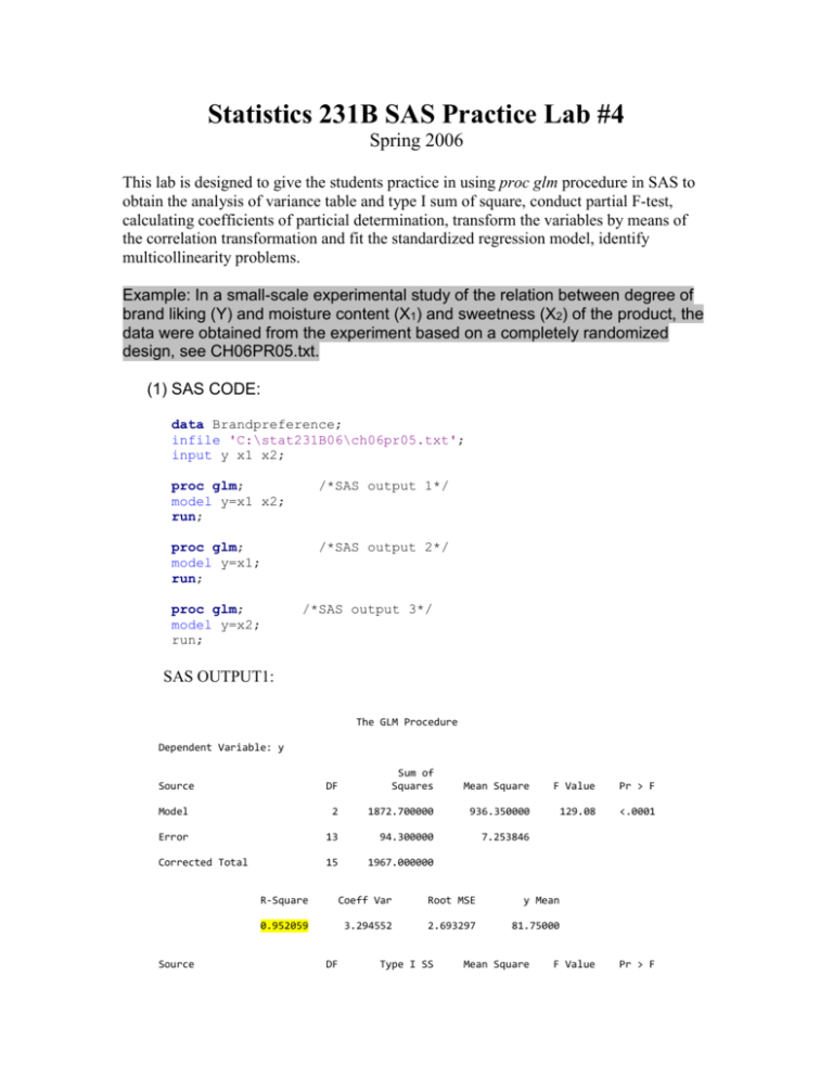
Statistics 231B SAS Practice Lab #4
Spring 2006
This lab is designed to give the students practice in using proc glm procedure in SAS to
obtain the analysis of variance table and type I sum of square, conduct partial F-test,
calculating coefficients of particial determination, transform the variables by means of
the correlation transformation and fit the standardized regression model, identify
multicollinearity problems.
Example: In a small-scale experimental study of the relation between degree of
brand liking (Y) and moisture content (X1) and sweetness (X2) of the product, the
data were obtained from the experiment based on a completely randomized
design, see CH06PR05.txt.
(1) SAS CODE:
data Brandpreference;
infile 'C:\stat231B06\ch06pr05.txt';
input y x1 x2;
proc glm;
model y=x1 x2;
run;
/*SAS output 1*/
proc glm;
model y=x1;
run;
/*SAS output 2*/
proc glm;
model y=x2;
run;
/*SAS output 3*/
SAS OUTPUT1:
The GLM Procedure
Dependent Variable: y
Source
DF
Sum of
Squares
Mean Square
F Value
Pr > F
Model
2
1872.700000
936.350000
129.08
<.0001
Error
13
94.300000
7.253846
Corrected Total
15
1967.000000
F Value
Pr > F
Source
R-Square
Coeff Var
Root MSE
y Mean
0.952059
3.294552
2.693297
81.75000
DF
Type I SS
Mean Square
x1
x2
Source
x1
x2
1
1
1566.450000
306.250000
1566.450000
306.250000
215.95
42.22
<.0001
<.0001
DF
Type III SS
Mean Square
F Value
Pr > F
1
1
1566.450000
306.250000
1566.450000
306.250000
215.95
42.22
<.0001
<.0001
Parameter
Estimate
Standard
Error
t Value
Pr > |t|
Intercept
x1
x2
37.65000000
4.42500000
4.37500000
2.99610324
0.30111971
0.67332413
12.57
14.70
6.50
<.0001
<.0001
<.0001
Question (1): From the above output, what is the extra sums of squares associated
with X1 , and with X2, given X1? Can X2 be dropped from the regression model given
that X1 is retained? Use the level of significance 0.01. State the alternative, decision
rule, and conclusion. What is the p-value of the test?
SAS OUTPUT 2:
The GLM Procedure
Dependent Variable: y
Source
DF
Sum of
Squares
Mean Square
F Value
Pr > F
Model
1
1566.450000
1566.450000
54.75
<.0001
Error
14
400.550000
28.610714
Corrected Total
15
1967.000000
R-Square
Coeff Var
Root MSE
y Mean
0.796365
6.542995
5.348898
81.75000
Source
x1
Source
x1
DF
Type I SS
Mean Square
F Value
Pr > F
1
1566.450000
1566.450000
54.75
<.0001
DF
Type III SS
Mean Square
F Value
Pr > F
1
1566.450000
1566.450000
54.75
<.0001
Parameter
Estimate
Standard
Error
t Value
Pr > |t|
Intercept
x1
50.77500000
4.42500000
4.39456848
0.59802502
11.55
7.40
<.0001
<.0001
Therefore, we can calculate R 2Y1 =1566.45/1967=0.7964,
R 2Y 2|1 
and
SSR (X 2 | X1 ) 306.25

 0.7645737
SSE (X1 )
400.55
SAS OUTPUT3:
The GLM Procedure
Dependent Variable: y
Source
DF
Sum of
Squares
Mean Square
F Value
Pr > F
Model
1
306.250000
306.250000
2.58
0.1304
Error
14
1660.750000
118.625000
Corrected Total
15
1967.000000
R-Square
Coeff Var
Root MSE
y Mean
0.155694
13.32295
10.89151
81.75000
Source
x2
Source
x2
DF
Type I SS
Mean Square
F Value
Pr > F
1
306.2500000
306.2500000
2.58
0.1304
DF
Type III SS
Mean Square
F Value
Pr > F
1
306.2500000
306.2500000
2.58
0.1304
Parameter
Estimate
Intercept
x2
68.62500000
4.37500000
Standard
Error
t Value
8.61049505
2.72287761
Pr > |t|
7.97
1.61
<.0001
0.1304
Question (2): Based on the above output, can you get R 2Y 2 =0.1557 and R2 =0.9521 (the
multiple coefficient of determination between Y and X1 and X2)?
2
Question (3): Using SAS code analog to above, how can you get R 12
( the simple
coefficient of determination between X1 and X2) and R 2Y1|2 ?
Another way to obtain R 2Y 2|1 is to use the following code:
data Brandpreference;
infile 'Z:\ch06pr05.txt';
input y x1 x2;
proc corr;
var y x2;
partial x1; /*calculate ry 2|1  R 2Y 2|1 */
run;
SAS OUTPUT 4:
1 Partial Variables:
2
Variables:
x1
y
x2
Simple Statistics
Variable
x1
y
x2
N
Mean
Std Dev
Sum
Minimum
Maximum
16
16
16
7.00000
81.75000
3.00000
2.30940
11.45135
1.03280
112.00000
1308
48.00000
4.00000
61.00000
2.00000
10.00000
100.00000
4.00000
Simple Statistics
Variable
Partial
Variance
Partial
Std Dev
x1
y
x2
28.61071
1.14286
5.34890
1.06904
Pearson Partial Correlation Coefficients, N = 16
Prob > |r| under H0: Partial Rho=0
y
x2
y
1.00000
0.87440
<.0001
x2
0.87440
1.00000
Therefore, R 2Y2|1  0.8744 ^2  0.7645737
Question (4): Using SAS code analog to the above, how can you get R 2Y1|2 ?
2
Question (5): Can you explain what R 2Y1 , R 2Y2 , R 12
, R 2Y1|2 , R 2Y2|1 , R 2 measures and interpret
your results?
(2) Use of the correlation transformation, which expresses the regression coefficients
in the same units, may be of help when these coefficients are compared and helps
with controlling roundoff errors. We first describe the correlation transformation
and then the resulting standardized regression model.
Ordinary multiple regression model: Yi   0  1 X i1   2 X i 2   i
 Yi  Y 


n  1  s Y 
1  X ik  X 
'


X ik

n  1  s X 
Yi' 
Correlation Transformation:
1
 (Y
i
sY 
sk 
 Y) 2
i
n 1
 (X
ik
 Xk )2
i
n 1
Standardized regression model: Yi'  1' X i'1   '2 X i' 2   i'
The relation between the ordinary multiple regression coefficients and the standardized
regression coefficients:
s 
 k   Y  'k (k  1,..., p - 1)
 sk 
 0  Y  1 X1     p 1 X p 1
We see that the standardized regression coefficients and the original regression
coefficients are related by simple scaling factors involving ratios of standard deviations.
Therefore, the return to the estimated regression coefficients for regression model in the
original variables is accomplished by employing the relations:
s 
b k   Y b 'k (k  1,..., p - 1)
 sk 
b 0  Y  b1 X1    b p 1 X p 1
For more details, please read page 271-278 of textbook ALSM.
SAS CODE:
data Brandpreference;
infile 'Z:\ch06pr05.txt';
input y x1 x2;
proc reg simple;
model y=x1 x2/stb; /fit the
run;
standardized regression*/
SAS OUTPUT 5:
Descriptive Statistics
Variable
Intercept
Sum
Mean
Uncorrected
SS
Variance
Standard
Deviation
16.00000
1.00000
16.00000
0
0
x1
x2
y
112.00000
48.00000
1308.00000
7.00000
3.00000
81.75000
864.00000
160.00000
108896
5.33333
1.06667
131.13333
2.30940
1.03280
11.45135
Parameter Estimates
Variable
DF
Parameter
Estimate
Standard
Error
t Value
Pr > |t|
Standardized
Estimate
Intercept
x1
x2
1
1
1
37.65000
4.42500
4.37500
2.99610
0.30112
0.67332
12.57
14.70
6.50
<.0001
<.0001
<.0001
0
0.89239
0.39458
Question (5) can you interpret the standardized regression coefficient 0.89239 and
0.39458? (please refer to the example on page 276-278).
Question (6) can you transform the estimated standardized regression coefficients by
means of (7.53) in the textbook ASLM back to the ones for the fitted regression
model in the original variables? Are they are equal to 4.425 and 4.375 respectively ?
(please also refer to the example on page 276-278).
(2) Multicollinearity issues
Question (7) Compare the estimated coefficient for moisture content (X1) obtained in
SAS OUTPUT 2 with the corresponding coefficient obtained in SAS OUPUT 1, what
do you find?
Question (8) Does SSR(X1) equal SSR(X1|X2) here?
2
Question (9) Refer to the R 12
you just obtained, what bearing does this have on your
findings in above two questions?
(3) Coefficient of Partial Correlation
The square root of a coefficient of partial determination is called a coefficient of
partial correlation. For more details, please see page 270-271 of textbook ASLM.
SAS CODE:
data Brandpreference;
infile 'Z:\ch06pr05.txt';
input y x1 x2;
proc reg data=Brandpreference;
model y=x2/P R; /*Regress Y on X2
and obtain residuals.*/
output out=result1 P=pred R=resid;
model x1=x2 /P R; /*Regress X1 on X2 and obtain
output out=result2 P= pred1 R=resid1;
run;
residuals.*/
proc sort data=result1; by y;run; /*sort result1 by Y*/
proc sort data=result2; by y;run; /*sort result2 by Y*/
data result; /*merge the two datasets together containing*/
/*one column of resid and one column of resid1*/
merge result1 result2;
by y;
run;
proc corr; /pearson correlation between resid and resid1*/
var resid resid1;
run;
DATA in result:
Obs
y
x1
x2
pred
resid
1
2
3
4
5
6
7
8
9
10
11
12
13
14
15
16
64
73
61
76
72
80
71
83
83
89
86
93
88
95
94
100
4
4
4
4
6
6
6
6
8
8
8
8
10
10
10
10
2
4
2
4
2
4
2
4
2
4
2
4
2
4
2
4
77.375
86.125
77.375
86.125
77.375
86.125
77.375
86.125
77.375
86.125
77.375
86.125
77.375
86.125
77.375
86.125
-13.375
-13.125
-16.375
-10.125
-5.375
-6.125
-6.375
-3.125
5.625
2.875
8.625
6.875
10.625
8.875
16.625
13.875
Obs
y
x1
x2
pred
resid
pred1
resid1
1
2
3
4
5
6
7
8
9
10
11
12
13
14
15
16
61
64
71
72
73
76
80
83
83
86
88
89
93
94
95
100
4
4
6
6
4
4
6
6
8
8
10
8
8
10
10
10
2
2
2
2
4
4
4
4
2
2
2
4
4
2
4
4
77.375
77.375
77.375
77.375
86.125
86.125
86.125
86.125
77.375
77.375
77.375
86.125
86.125
77.375
86.125
86.125
-16.375
-13.375
-6.375
-5.375
-13.125
-10.125
-6.125
-3.125
5.625
8.625
10.625
2.875
6.875
16.625
8.875
13.875
7
7
7
7
7
7
7
7
7
7
7
7
7
7
7
7
-3
-3
-1
-1
-3
-3
-1
-1
1
1
3
1
1
3
3
3
SAS OUTPUT 6:
Pearson Correlation Coefficients, N = 16
Prob > |r| under H0: Rho=0
resid
resid1
resid
Residual
1.00000
0.97119
<.0001
resid1
Residual
0.97119
<.0001
1.00000
Question (10) : Does the pearson correlation coefficient between resid and resid1 0.97119
equal to rY1|2 ?( you can use the code for SAS OUTPUT 4 to get the value for rY1|2 ).