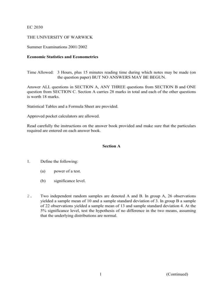
EC 2030
THE UNIVERSITY OF WARWICK
Summer Examinations 2001/2002
Economic Statistics and Econometrics
Time Allowed: 3 Hours, plus 15 minutes reading time during which notes may be made (on
the question paper) BUT NO ANSWERS MAY BE BEGUN.
Answer ALL questions in SECTION A, ANY THREE questions from SECTION B and ONE
question from SECTION C. Section A carries 28 marks in total and each of the other questions
is worth 18 marks.
Statistical Tables and a Formula Sheet are provided.
Approved pocket calculators are allowed.
Read carefully the instructions on the answer book provided and make sure that the particulars
required are entered on each answer book.
Section A
1.
2.
Define the following:
(a)
power of a test.
(b)
significance level.
Two independent random samples are denoted A and B. In group A, 26 observations
yielded a sample mean of 10 and a sample standard deviation of 3. In group B a sample
of 22 observations yielded a sample mean of 13 and sample standard deviation 4. At the
5% significance level, test the hypothesis of no difference in the two means, assuming
that the underlying distributions are normal.
1
(Continued)
EC 2030
3.
Calculate the approximate power of the t-test calculated in question 2, given that
A-B=-3.0. What is the Type I error for this test?
4.
For the following regression model, estimated using annual data from 1940 to 1999,
Y t  0.021  0.920 X t  e t
(0.038)
(standard error in parentheses)
5.
(a)
Test at the 5% significance level that the slope coefficient is unity.
(b)
What is the forecast for year 2000, given that X2000 = 4.1?
(c)
A dummy variable Dt is added to the equation, taking value unity in 2000 and
zero otherwise. The regression is re-estimated over the period 1940 to 2000
using the data point X2000 = 4.1, but data for Y2000 is unavailable so the
researcher simply inputs a zero value for Y2000. Interpret the coefficient on Dt.
Consider the following regression model:
Yt  1   2 X 1t   3 X 2 t   t
rearranging equation (1) we get:
(1)
Yt  X 2 t   1   2 ( X 1t  X 2 t )   3 X 2 t   t
(2)
(a)
Express each of the parameters,  1 ,  2 ,  3 as a function of 1 ,  2 ,  3
(b)
Hence or otherwise show how one can test the hypothesis  2   3  1 using
only equation 2.
2
(Continued)
EC 2030
6.
Estimating a model by OLS for imports (m) against relative prices (domestic
prices/foreign prices) (p/p*), and real GDP (y) for the UK using quarterly data over the
period 1978:1 to 1997:4 yielded the results:
ln( mt )  0.045  0.5 ln( p t / p t* )  0.6 ln( y t )  e t
(0.042) (0.125)
(0.201)
(1)
, ln = natural log
.
R2  0.962 , SSE  0147
(standard errors in parentheses)
(a)
(b)
7.
Calculate the power of the test (at the 5% significance level) that the coefficient
on the variable ln(y) is zero, given that the true coefficient is 0.3.
1 t  1994 : 1  1997 : 4
The variable ln( p t / p*t ) * D t , where D t  
, is added to
otherwise
0
equation (1), which is then re-estimated. Interpret the coefficients of this new
equation.
Explain what the implications on the properties of the OLS estimators are for each
of the following:
(a) Omitted relevant variables.
(b) An outlier in one of the explanatory variables.
3
(Continued)
EC 2030
Section B
8.
(a)
The West Anglia Great Northern Railway (WAGN) and Chiltern Railways
(Chiltern) have both attempted to prevent recent rail maintenance work leading
to an increase in rail journey time. A random sample of 100 rail journeys were
taken for each company. For WAGN, the average journey time rose by 3
minutes, with a standard deviation of 15.5, whereas for Chiltern the average
journey time rose by 1.3 minutes, with a standard deviation of 16.1.
At the 5% significance level:
(b)
(i)
Separately test whether WAGN and Chiltern have been successful in
preventing increased journey times. Write a sentence summarising the
findings of these tests.
(ii)
Test whether WAGN has been more successful than Chiltern in
preventing an increase in journey time.
In 1994 two American economists claimed that male catering staff earned more
than females performing the same job. A random sample of 50 female catering
staff was found to earn an average of $16,000, with a standard deviation of
$2,600, while a sample of 40 male catering staff was found to earn an average of
$17,300, with a standard deviation of $3,000.
(i)
What is the power of a test at the 5% level of the American economists’
claim, given that male catering staff are truly paid £100 more than
female catering staff?
(ii)
Diagramatically represent the power and significance level of the test
conducted in (b) (i).
(ii)
At the 10% level, is there a significant difference between the two groups
in the variance of earnings?
4
(Continued)
EC 2030
9.
The following estimated equation was obtained by Ordinary Least Squares using
quarterly data for the period 1963:3-1992:4 inclusive:
y t  0.010  0.209 w t  0189
. x t  0187
. zt  et
(0.072) (0.058) (0.088)
Regression Sum of Squares (SSR) = 0.0035, Error Sum of Squares (SSE) = 0.0157
(standard errors are given in parentheses)
(a)
Test whether each of the coefficients are significantly different from zero at
both the 5% and 1% significance level.
(b)
Calculate (i) the coefficient of determination (R2) and (ii) the standard error
(  ) of the regression.
(c)
Test the significance of the regression.
(d)
Test the hypothesis that the coefficient on wt is equal and opposite to that on
zt, given that the covariance between the coefficients is -0.0015. Why might
the researcher want to impose this restriction?
(e)
Given that z t  w 3t , test the hypothesis that the marginal response of yt to wt is
zero at w t  1 , given that the covariance between the coefficients is-0.0015.
(f)
Without assuming any particular relationship between the variables, calculate
the SSE of the following restricted version of the model:
y t   0   1w t   2 x t  e t .
5
(Continued)
EC 2030
10.
A researcher collected seasonally adjusted quarterly data for the UK over the period
1979:1 to 2001:4 on the three variables
Lm = Natural log of real broad money (M3)
Ly = Natural log of real Gross Domestic Product (GDP)
r = 3 month Treasury bill rate
Table 1 contains the results, as reported by PcGive, for a money demand equation for
the UK using quarterly data over the period 1980:1-1999:4.
(i)
Provide answers for the 6 spaces, marked ??(x) in Table 1.
(ii)
Using the results of Table 1 and Figure 1, explain how you would proceed from
this initial general regression model to a more appropriate and parsimonious
model.
(iii)
Explain what other tests you might think of using to test the validity of your
preferred model.
TABLE 1
EQ(1) Modelling Lm by OLS
Variable
Coefficient
Constant
1.9304
Ly
0.1642
Ly_1
0.2287
Ly_2
0.2056
Ly_3
-0.1056
R
-0.0131
r_1
-0.0123
r_2
0.0098
r_3
-0.003
Lm_1
0.4532
Lm_2
-0.1921
Lm_3
0.0765
sigma
??(c)
R^2
??(d)
log-likelihood
-112.858
no. of observations
80
mean(y)
4.4986
AR 1- 4:
ARCH 4:
Normality:
Hetero Test:
RESET:
t-value
t-prob
1.961
0.050
1.462
??(a)
1.872
0.061
1.553
0.120
0.337
??(b)
-1.351
0.177
-1.352
0.176
0.961
0.337
-0.303
0.762
2.997
0.003
-1.296
0.195
0.617
0.537
RSS
0.02886
F(11,68) = ??(e) [0.000]**
DW
2.16
no. of parameters
12
var(y)
0.00201
F(4,64) = 1.0382[0.394]
F(4,60) =
2.283[0.071]
2
Chi (2)= 15.197[??(f)]***
F(22,45) = 1.2019[0.294]
F(1,67) = 0.03373[0.855]
(Question 10 continued overleaf)
6
(Continued)
EC 2030
(Question 10 continued)
Figure 1:
4
Lm ´ Fitted
r:Lm (scaled)
4.6
2
4.5
0
4.4
-2
4.35
4.40
Density
r:Lm
4.45
4.50
4.55
4.60
1.0
N(0,1)
ACF-r:Lm
0.5
0.4
0.0
0.2
-0.5
-2
0
2
4
7
0
5
10
(Continued)
EC 2030
11.
A model is specified as
y t     1 x1,t   2 x1,t 1   3 x 2,t 1   4 x 2,t  2   5 y t  2   t (1)
Estimating this model using quarterly data over the period 1983:1-2000:4 resulted in
y t  0.424  0.624 x1,t  0.361x1,t 1  0.618 x 2,t 1  0.381x 2,t  2
(0.201) (0.168)
0.576 y t  2  et
(0.152)
(0.202)
(0.189)
(0.229)
R  0.705, Error sum of squares (SSE)  39.172
(Standard errors in parentheses)
2
(a)
Calculate the response in y to a unit increase in x1 and x2, (i) contemporaneously,
(ii) after 1 period, (iii) after 2 periods, (iv) after 3 periods, (v) in the long run.
(b)
Test the hypothesis that the long run response of y to x1 is –0.5, given that
cov( b1 , b 2 )  0.020 , cov( b1 , b5 )  0.01 and cov( b 2 , b5 )  0.009 .
(c)
Write out the restricted model that you would estimate in PcGIVE if you wanted
to impose the two hypotheses that the long-run coefficient on x1 is –1 and the
long-run coefficient on x2 is zero. How many parameters would you estimate in
the restricted model?
(d)
The Durbin-Watson statistic for the estimated equation (1) is 1.316. Based on
this information what do you conclude about the model (1)?
(e)
Describe the regressions you would run in order to construct the AR1-4 test
reported by PcGIVE. The p-value on the resultant F-statistic was 0.02. In light of
this information and that in (d) how would you suggest modifying equation (1)?
8
(Continued)
EC 2030
12.
An equation to determine happiness from a random sample of 600 employed individuals
is estimated based on the following model
ln( Happy i )    1 ln( Income i )   2 Female i   3 Married i   4 SOCIi
(1)
  5SOCIIi   6SOCIII i   7 SOCIVi   8 Educ i   9 Age   i
where,
Happy = Happiness score (out of 100)
Income=Annual income (£000s)
Educ = Number of years in education
Age = Age
1 fe male
1 Married
, Married i  
,
Female i  
0 male
0 Otherwise
1
SOCI i  
0
1 Managerial
1 Skilled
1
, SOCIII i  
, SOCIVi  
SOCII i  
0 Otherwise
0 Otherwise
0
1 Unskilled
.
SOCVi  
0 Otherwise
Pr ofessional
,
Otherwise
Semi - Skilled
,
Otherwise
Estimating equation (1) by OLS resulted in an error sum of squares (SSE) of 6.37 and a
regression sum of squares (SSR) of 2.72.
(a)
Excluding the variables SOCI, SOCII, SOCIII and SOCIV from equation (1) and
estimating the resultant equation by OLS, yielded an SSR of 2.48. Test the joint
significance of these variables.
(b)
The Standard Industrial Classifications (SIC) defines nine single digit industry
types. Explain how you would include variable(s) to control for the different
industry types in equation (1). Estimating equation (1) by OLS with the inclusion
of the industry variable(s) the SSE fell to 6.08. Test the significance of this
(these) variable(s).
(c)
Equation (1) is re-estimated separately for the 278 males and the 322 females in
our sample. Estimating these two models yielded SSEs of 3.13 and 3.02,
respectively. Comparing this model with equation (1), carefully explain what
null hypothesis you are testing, and test this hypothesis.
(d)
Adding three interacted dummy variables to equation (1), (Female)´(Educ),
(Female)´(Age) and (Female)´ln(Income) the SSE fell to 6.18. Test the joint
significance of these additional variables.
(e)
Compare the model estimated in (d) with the two models estimated in (c). Write
out the restrictions you must impose on the model described in (c) to produce the
model in (d) and test the restrictions.
9
(Continued)
EC 2030
13.
Consider the following model:
y t    1 ln( x 1t )   2 x 2 t  u t ,t  1, , n
(1)
(a)
Interpret the coefficients in equation (1)
(b)
Interpret the coefficient on the variable ln(x1t) in (1) if this variable is multiplied
by 100.
Discuss the consequences of estimating equation (1) by OLS, in terms of the OLS
estimators, b1 and b2, and the standard errors of these estimators, in each of the following
circumstances:
(c)
ut is serially correlated, when x2t = yt-1.
(d)
x 2t = [ln(x 1t )]2
(e)
x2t is unobservable and is therefore excluded from the estimated equation.
(f)
t  1,  n 1
1
. How could you improve upon OLS in this case?
V(u t ) = 
2 t  n 1  1 n
(g)
0
x 2t = 
1
t  1, 16,18,  n
.
t  17
Section C
14.
Blundell et al (2000) show that average earnings for both males and females who went
to university are markedly greater than those individuals who did not attend university.
Discuss this statement in the light of the statistical evidence on the returns to a university
degree.
15
Econometric models enable us to test competing economic theories against actual
data. Economic models which prove to be data inconsistent can then be discarded and
more appropriate models developed. Discuss.
10
(End)