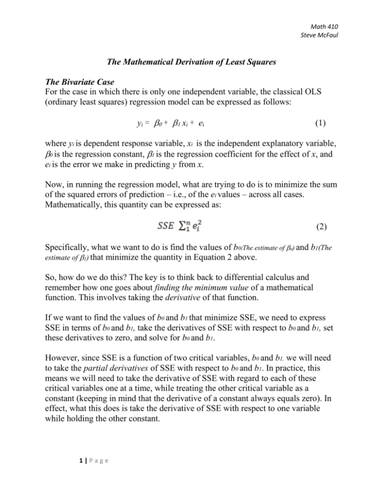
Math 410
Steve McFaul
The Mathematical Derivation of Least Squares
The Bivariate Case
For the case in which there is only one independent variable, the classical OLS
(ordinary least squares) regression model can be expressed as follows:
yi =  +  xi + ei
(1)
where yi is dependent response variable, xi is the independent explanatory variable,
0 is the regression constant, 1 is the regression coefficient for the effect of x, and
ei is the error we make in predicting y from x.
Now, in running the regression model, what are trying to do is to minimize the sum
of the squared errors of prediction – i.e., of the ei values – across all cases.
Mathematically, this quantity can be expressed as:
(2)
Specifically, what we want to do is find the values of b0(The estimate of 0) and b1(The
estimate of 1) that minimize the quantity in Equation 2 above.
So, how do we do this? The key is to think back to differential calculus and
remember how one goes about finding the minimum value of a mathematical
function. This involves taking the derivative of that function.
If we want to find the values of b0 and b1 that minimize SSE, we need to express
SSE in terms of b0 and b1, take the derivatives of SSE with respect to b0 and b1, set
these derivatives to zero, and solve for b0 and b1.
However, since SSE is a function of two critical variables, b0 and b1, we will need
to take the partial derivatives of SSE with respect to b0 and b1. In practice, this
means we will need to take the derivative of SSE with regard to each of these
critical variables one at a time, while treating the other critical variable as a
constant (keeping in mind that the derivative of a constant always equals zero). In
effect, what this does is take the derivative of SSE with respect to one variable
while holding the other constant.
1|Page
Math 410
Steve McFaul
We begin by rearranging the basic OLS equation for the bivariate case so that we
can express ei in terms of yi, xi, b0, and b1. This gives us:
ei  yi  b0  b1 xi
(3)
Substituting this expression back into Equation (2), we get
n
SSE   ( yi  b0  b1 xi ) 2
(4)
1
where n = the sample size for the data. It is this expression that we actually need to
differentiate with respect to b0 and b1. Let’s start by taking the partial derivative of
SSE with respect to the regression constant, b0, i.e.,
SSE
 n


( yi  b0  b1 x1 ) 2 


b0
b0  1

In doing this, we can move the summation operator (Σ) out front, since the
derivative of a sum is equal to the sum of the derivatives:

SSE n  
 
( yi  b0  b1 x1 ) 2 
b0
1  b0

We then focus on differentiating the squared quantity in parentheses. Since this
quantity is a composite – we do the math in parentheses and then square the result
– we need to use the chain rule in order to obtain the partial derivative of SSE with
respect to the regression constant. In order to do this, we treat yi, b1, and xi as
constants. This gives us:
SSE n
   2( yi  b0  b1 x1 )
b0
1
Further rearrangement gives us a final result of:
n
SSE
 2 ( yi  b0  b1 x1 )
b0
1
2|Page
(5)
Math 410
Steve McFaul
For the time being, let’s put this result aside and take the partial derivative of SSE
with respect to the regression coefficient, b1, i.e.,
SSE
 n


( yi  b0  b1 x1 ) 2 


b1
b1  1

Again, we can move the summation operator (Σ) out front:

SSE n  
 
( yi  b0  b1 x1 ) 2 
b1
1  b10

We then differentiate the squared quantity in parentheses, again using the chain
rule. This time, however, we treat yi, b0, and xi as constants. With some subsequent
rearrangement, this gives us:
n
SSE
 2 xi ( yi  b0  b1 x1 )
b1
1
(6)
With that, we have our two partial derivatives of SSE – in Equations (5) and (6)
The next step is to set each one of them to zero:
n
0  2 ( yi  b0  b1 x1 )
(7)
1
n
0  2 xi ( yi  b0  b1 x1 )
(8)
1
Equations (7) and (8) form a system of equations with two unknowns – our OLS
estimates, b0 and b1. The next step is to solve for these two unknowns. We start by
solving Equation (7) for b0. First, we get rid of the -2 by multiplying each side of
the equation by -1/2:
n
0   ( yi  b0  b1 x1 )
1
3|Page
Math 410
Steve McFaul
Next, we distribute the summation operator though all of the terms in the
expression in parentheses:
n
n
n
1
1
1
0   yi   b0   b1 x1
Then, we add the middle summation term on the right to both sides of the equation,
giving us:
n

n
n
1
1
b0   yi   b1 x1
1
Since b0 and b1 the same for all cases in the original OLS equation, this further
simplifies to:
n
n
1
1
nb0   yi   b1 x1
To isolate b0 on the left side of the equation, we then divide both sides by n:
n
b0 
y
1
1
n
n
 b1
x
i
1
(9)
n
Equation (9) will come in handy later on, so keep it in mind. Right now, though, it
is important to note that the first term on the right of Equation (9) is simply the
mean of yi, while everything following b1 in the second term on the right is the
mean of xi.
b0  y  b1 x
(10)
Now, we need to solve Equation (8) for b1. Again, we get rid of the -2 by
multiplying each side of the equation by -1/2:
n
0   xi ( yi  b0  b1 x1 )
1
4|Page
Math 410
Steve McFaul
Next, we distribute xi through all of the terms in parentheses:
n
0   xi yi  xi b0  b1 xi2 )
1
We then distribute the summation operator through all of the terms in the
expression in parentheses:
n
n
n
1
1
1
0   xi yi   xi b0   b1 xi2
Next, we bring all of the constants in these terms (i.e., b0 and b1) out in front of the
summation operators, as follows:
n
n
n
1
1
1
0   xi yi  b0  xi  b1  xi2
We then add the last term on the right side of the equation to both sides:
n
n
n
1
1
b1  x   xi yi  b0  xi
2
i
1
Next, we go back to the value for b0 from Equation (9) and substitute it into the
result we just obtained. This gives us:
n
b1 
1
n
 n

xi  n

n
  yi
xi2   xi yi   1
 b1 1   xi
n  1
 n
1


Multiplying out the last term on the right, we get:
 n 2 
1 yi 1 xi   1 xi  
n
2
xi   xi y i 
 b1


n
n
1




n
n
b1 
1
5|Page
n
Math 410
Steve McFaul
If we then add the last term on the right to both sides of the equation, we get:
n
b1 
1
n
n
 n 2 
   xi   n
y
1 i 1 xi
1


2


xi  b1
 xi yi 

 
n
n
1




On the left side of the equation, we can then factor out b1:
2
n
n

 n  
  xi   n
n
y
1 i 1 xi
1


2


b1  xi 
 xi y i 
1
 
n
n
1




If we divide both sides of the equation by the quantity in the large brackets on the
left side, we can isolate b.
n
b1 
x y
i
i

n
n
1
1
 y i  xi
n
1
n

1
 n 
  xi 
xi2   1 
n
2
Finally, if we multiply top and bottom by n we obtain the least-square estimator for
the regression coefficient in the bivariate case. This is the form from lecture:
n
b1 
n
n xi yi   yi  xi
1
1
n
n
1
6|Page
n
1


x    xi 
 1 
n
2
i
2
(11)
Math 410
Steve McFaul
The Multiple Regression Case: Deriving OLS with Matrices
The foregoing math is all well and good if you have only one independent variable
in your analysis. However, in practice, this will rarely be the case: rather, we will
usually be trying to predict a dependent variable using scores from several
independent variables. Deriving a more general form of the least-squares estimator
for situations like this requires the use of matrix operations. The basic OLS
regression equation can be represented in the following matrix form:
Y = XB + e
(12)
where Y is an n×1 column matrix of cases’ dependent variable, X is an n×(k+1)
matrix of cases’ scores on the independent variables (where the first column is a
placeholder column of ones for the constant and the remaining columns correspond
to each independent variable), B is a (k+1) column matrix containing the
regression constant and coefficients, and e is an n×1 column matrix of cases’
errors of prediction. As before, what we want to do is find the values for the
elements of B that minimize the sum of the squared errors. The quantity that we
are trying to minimize can be expressed as follows:
SSE = e′e
(13)
If you work out the matrix operations for the expression on the right, you’ll notice
that the result is a scalar – a single number consisting of the sum of the squared
errors of prediction (i.e., multiplying a 1×N matrix by a N×1 matrix produces a
1×1 matrix, i.e., a scalar). In order to take the derivative of the quantity with regard
to the B matrix, we first of all need to express e in terms of Y, X, and B:
e = Y – XB
Substituting the expression on the right side into Equation (13), we get:
SSE =(Y − XB)′(Y − XB)
Next, the transposition operator on the first quantity in this product (Y - XB)′ can
distributed:
SSE =
(Y′
− B′X′)(Y − XB)
When this product is computed, we get the following:
SSE = Y′Y − Y′XB − B′X′Y + B′X′XB
7|Page
Math 410
Steve McFaul
Now, if multiplied out, the two middle terms Y′XB and B′X′Y are identical: they
produce the same scalar value. As such, the equation can be further simplified to:
SSE = Y′Y − 2Y′XB + B′X′XB
(14)
We now have an equation which expresses SSE in terms of Y, X, and B. The next
step , as in the bivariate case, is to take the derivative of SSE with respect to the
matrix B.
SSE
 (Y Y  2Y XB  BX XB)
B
First, since we are treating all matrices besides B as the equivalent of constants, the
first term in parentheses – based completely on the Y matrix – has a derivative of
zero. Second, the middle term – known as a “linear form” in B – is the equivalent
of a scalar term in which the variable we are differentiating with respect to is raised
to the first power (i.e. a linear term), which means we obtain the derivative by
dropping the B and taking the transpose of all the matrices in the expression which
remain, giving us -2X′Y.
Finally, the third term – known as a “quadratic form” in B – is the equivalent of a
scalar term in which the variable we are differentiating with respect to is raised to
the second power (i.e., a quadratic term). This means we obtain the derivative by
dropping the B′ from the term and multiplying by two, giving us 2X′XB. Thus, the
full partial derivative is
SSE
 (2 X 'Y  2 X XB)
B
(15)
The next step is to set this partial derivative to zero and solve for the matrix B.
This will give us an expression for the matrix of estimates that minimize the sum
of the squared errors of prediction. We start with the following:
0 = −2X′Y + 2X′XB
We then subtract 2X′XB from each side of the equation:
− 2X′XB = −2X′Y
8|Page
Math 410
Steve McFaul
Next, we eliminate the -2 on each term by multiplying each side of the equation by
-1/2:
X′XB = X′Y
Finally, we need to solve for B by pre-multiplying each side of the equation the
inverse of (X′X), i.e., (X′X)-1. Remember that this is the matrix equivalent of
dividing each side of the equation by (X′X):
B=
(X′X)-1
X′Y
(16)
Equation (16) is the OLS estimator. To tie this back to the bivariate case, note
closely what the expression on the right does. While X′Y gives the sum of the
cross-products of X and Y, X′X gives us the sum of squares for X. Since premultiplying X′Y by (X′X)-1 is the matrix equivalent of dividing X′Y by X′X, this
expression is basically doing the same thing as the scalar expression for b1 in
Equation (11): dividing the sum of the cross products of the IV (or IVs) and the
DV by the sum of squares for the IV (or IVs).
9|Page