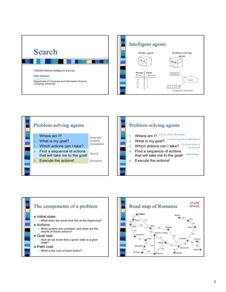
Intelligent agents
Search
Reflex agent
Problem-solving
agent
TDDC65 Artificial intelligence and Lisp
Percept Action
If I see… …then I do:
Peter Dalenius
petda@ida.liu.se
Department of Computer and Information Science
Linköping University
A
B
C
D
Problem
2
1
1
3
Search
2, 3, 1, 4, 4, 1
A sequence of actions
Problem-solving agents
1.
2.
3.
4.
5.
Where am I?
What is my goal?
Which actions can I take?
Find a sequence of actions
that will take me to the goal!
Execute the actions!
Problem-solving agents
Goal and
problem
formulation
Search
Execution
The components of a problem
I’m in Arad, Romania.
Where am I?
I want to go go to Bucharest.
What is my goal?
Go from town A
Which actions can I take?
to town B.
Find a sequence of actions
that will take me to the goal! Searching…
Execute the actions!
1.
2.
3.
4.
5.
Oradea
Initial
state
– What does the world look like at the beginning?
Actions
– What actions are available, and what are the
results of these actions?
Goal
test
– How do we know that a given state is a goal
state?
Path
cost
– What is the cost of each action?
STATE
SPACE
Road map of Romania
Neamt
71
75
87
Iasi
151
Zerind
92
Arad
140
Sibiu
Fagaras
99
118
80
Rimnicu Vilcea
142
Timisoara
211
Lugoj
111
97
146
Mehadia
85
101
138
75
Urziceni
Pitesti
70
Drobeta
Vaslui
120
Craiova
Hirsova
98
86
Bucharest
90
Eforie
Giurgiu
1
Romanian route finding
The initial state
Arad
After expanding Arad
Arad
SEARCH
SPACE
Some definitions
– state – a description of (some aspect of) the world
configuration
– action – changes the world from one state to
another
– state space – the set of all possible states
EXPANDED
GENERATED
Sibiu
Timisoara
Sibiu
Arad
Oradea
Fagaras
Zerind
Arad
After expanding Sibiu
Timisoara
Rimnicu
Vilcea
Zerind
FRINGE
General search algorithm
The static part (problem definition)
The dynamic part (search for solution)
– search space – the result of exploring all possible
actions
– node – a part of the search space, corresponding
to a state, but contains more information
Example: Crossing the river
function TREE-SEARCH(problem, fringe) returns a solution or failure
fringe ← INSERT(MAKE-NODE(INITIAL-STATE[problem]), fringe)
loop do
if EMPTY?(fringe) then
return failure
node ← REMOVE-FIRST(fringe)
if GOAL-TEST[PROBLEM](STATE[node]) then
return SOLUTION(node)
fringe ← INSERT-ALL(EXPAND(node, problem), fringe)
• Everything must cross the river.
• Only one thing can fit in the boat, besides the farmer.
• The lamb will eat the cabbage, and the wolf will eat
the lamb, if left alone.
START
Problem formulation
Initial
FW | LC
state
– Everything to the right
STATE
SPACE
| FWLC
FL | WC
FC | WL
F | WLC
| FWLC
L
| FWC
Actions
– Farmer and maximum one passenger may cross
Goal
| FC
FWL | C
FLC | W
LC
| FW
test
– Everything to the left
Path
WL
FWLC |
W
| FLC
C
| FWL
cost
– Each step costs 1
FWC | L
WC
| FL
FWLC |
2
Search strategies
A strategy is defined by picking the order of
node expansion.
Strategies are evaluated by:
–
–
–
–
Classes of search strategies
Completeness: Does it always find a solution, if one exists?
Time complexity: Number of nodes generated
Space complexity: Maximum number of nodes in memory
Optimality: Does it always find the cheapest solution?
Time and space complexity are measured by:
– b (maximum branch factor of the search tree)
– d (depth of the cheapest solution)
– m (maximum depth of the state space, possibly infinite)
1. Bredth-first search
Uninformed
Informed
Bredth-first search
all nodes at level n before
expanding nodes at level n+1
Generated nodes are placed in a FIFO
queue (first in, first out)
Bredth-first search
D
A
B
B
C
C
remove here
A
FIFO Queue
insert here
FIFO Queue
E
D
C
E
FIFO Queue
Bredth-first search
C D
B
search (heuristic search)
– Strategies have additional information
whether non-goal states are more
promising than others
Expand
A
search (blind search)
– No additional information besides what is
in the problem definition
– Can only generate successor states and
compare against goal state
B
D
E
F
G
C
E
F
G
3
Analysis of bredth-first search
BFS space and time complexity
Complete?
– Yes, we will always find a solution, provided that
the branching factor b is finite.
–
–
–
–
Optimal?
– Yes, if the path cost is a nondecreasing function of
the node depth (e.g. when path cost is uniform).
Space
complexity?
– O(bd+1)
Time
complexity?
Branching factor b
Root: one node
Level 1: b nodes
Level 2: b2 nodes
Level n: bn nodes
Assume that the goal is at level d
The number of nodes processed is
1 + b + b2 + b3 + … + bd + (bd+1-b) = O(bd+1)
– O(bd+1)
Complexity analysis
Big O notation or Ordo notation is used in
complexity analysis to indicate the most
important factor.
T(n) = O(f(n))
if T(n) < kf(n) for some k, for all n > n0
If time complexity is O(n2) this means that for
some k the time used will always be less than
kn2.
Big O notation gives a rough answer to the
question How bad can it be?
2. Depth-first search
Always
Extension: Uniform-cost search
Always
expand the node with the lowest
path cost
Complete and optimal if the cost of each
action is at least ε (i.e. no ”free” actions)
Depth-first search
insert here
expand the deepest node in the
fringe
Generated nodes are placed in a LIFO
queue or stack (last in, first out)
A
LIFO Queue (Stack)
B
B
C
C
remove here
4
Depth-first search
A
Depth-first search
D
C
B
D
A
LIFO Queue (Stack)
E
H
E
C
B
D
E
H
Depth-first search
A
D
H
CI
E
C
C
E
I
Analysis of depth-first search
LIFO Queue (Stack)
EI
B
LIFO Queue (Stack)
C
C
E
C
C
E
Complete?
– No, if the tree has infinite depth we will never get
an answer.
Optimal?
– No. If the optimal goal is in the right subtree, we
will find any non-optimal goals in the left part first.
Space
I
complexity?
– O(bm)
Time
complexity?
– O(bm)
DFS time and space complexity
Extension: Depth-limited search
How
Introduce
many nodes must
be kept in memory?
– All unexpanded nodes,
b nodes at each level.
In total: bm + 1 = O(bm)
How
many nodes must be accessed?
– In the worst case, all nodes in the tree.
In total: bm = O(bm)
a depth limit l and treat nodes
at depth l as if they have no successors.
Not complete or optimal, but at least we
can guarantee that the algorithm does
not get stuck in an infinite loop.
Can be useful if we know something
about the problem that can help us
choose l.
5
3. Iterative deepening search
4. Bidirectional search
Combines
the benefits of bredth-first
and depth-first.
Does a depth-limited search with
increasing depth limit l until a goal is
found.
Two
Uninformed search strategies
Informed search strategies
simultaneous searches: one from
the intitial state, one from the goal state
and backwards
Reduced complexity
How can we search backwards?
Bredthfirst
Uniformcost
Depthfirst
Depthlimited
Iterative
deepening
Bidirectional
Complete
Yes 1
Yes 1,2
No
No
Yes 1
Yes 1,4
Optimal
Yes 3
Yes
No
No
Yes 3
Yes 3,4
Time
O(bd+1)
O(b1+k)
O(bm)
O(bl)
O(bd)
O(bd/2)
Space
O(bd+1)
O(b1+k)
O(bm)
O(bl)
O(bd)
O(bd/2)
Use problem-specific knowledge beyond the
problem definition itself.
Always select the ”best” node, based on an
evaluation function f(n).
The additional information encoded in the
evaluation function is called a heuristic (rule
of thumb, way of making educated guesses).
Different informed search strategies use
different heuristics.
m = max depth, l = depth limit
1) if b is finite 2) if step cost ≥ ε 3) if uniform step cost
4) if both directions use bredth-first search
b = branching factor, d = depth of goal
5. Greedy best-first search
to expand the node that we
currently believe is closest to a goal.
Uses the following heuristic:
Greedy best-first search
Tries
– h(n) = estimated cost of the cheapest path from
node n to a goal node
A
B
65
78
C
Priority queue
54
C
B
54
65
remove here
insert here
(sorted)
6
Greedy best-first search
Example: Romanian road trip
Arad
A
78
Sibiu
B
C
65
54
B
F
G
B
44
65
51
65
remove here
F
366
Priority queue
G
44
insert here
(sorted)
51
Arad
Oradea
366
380
Timisoara 329
253
Fagaras
Zerind
374
Rimnicu
Vilcea
176
193
Sibiu
Bucharest
253
0
Stages in a greedy best-first search for Bucharest using the straight-line distance heuristic.
Analysis of greedy best-first search
6. A* search
Complete?
Same
Optimal?
– No. Just like depth-first search we will try to follow
a single path and backtrack when we hit a dead
end.
Space
Time
complexity?
complexity?
– O(bm)
– With a good heuristic this can be reduced, but the
worst case is the same as for depth-first search.
Example: Romanian road trip
Arad
Sibiu
393=140+253
Arad
Oradea
Fagaras
646=
280+366
671=
291+380
415=
239+176
basic principle as greedy bestfirst search
Uses the heuristic g(n) + h(n)
– g(n) = the cost to reach node n
– h(n) = estimated cost of the cheapest path from
node n to a goal node
Pronounced
”A-star”
Proof that A* is optimal
Will n or G2 be expanded?
366=0+366
Timisoara
Zerind
447=118+329
449=75+374
f(n) = g(n)+h(n) ≤ g(G1)
f(G2) = g(G2)+h(G2) = g(G2) > g(G1)
n
Rimnicu
Vilcea
413=
220+193
Sibiu
Bucharest
591=
338+253
450=
450+0
Stages in an A* search for Bucharest.
G2
suboptimal
goal
Craiova
Pitesti
Sibiu
526=
366+160
417=
317+100
553=
300+253
Bucharest
Craiova
R. Vilcea
418=
418+0
615=
455+160
607=
414+193
G1
optimal
goal
If h(n) never overestimates the cost, then A* is optimal.
We call h(n) an admissible heuristic.
7