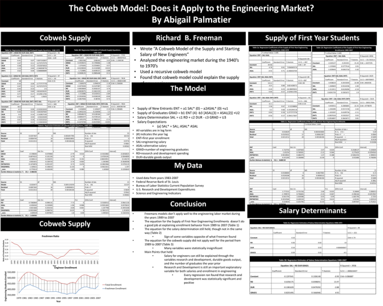
The Cobweb Model: Does it Apply to the Engineering Market?
By Abigail Palmatier
Cobweb Supply
Richard B. Freeman
Equation: Ent = GRAD RD DUR ASAL ENT1 ENT2
R-Squared = .97
Coefficient Standard Error T-Statistic
S.E.E. = .50
Constant
18
D.W.=2.21
GRAD
-0.34
0.09 -3.777777778
RD
0.47
0.11 4.272727273
DUR
0.35
0.14
2.5
ASAL
-1.87
0.49 -3.816326531
ENT1
0.77
0.17 4.529411765
ENT2
-0.17
0.16
-1.0625
Equation: Ent = GRAD RD DUR ASAL ENT1 ENT2
R-Squared = .7818
Coefficient
Standard Error
T-Statistic S.E.E. = .004631382
Constant
2.383079
1.094019
2.18 D.W.=1.258304
GRAD
0.3270326
0.2147387
1.52
RD
0.9920839
0.2656157
3.74
DUR
-0.0658375
0.1661319
-0.4
ASAL
-1.515086
0.5333412
-2.84
ENT1
-0.1934356
0.4246539
-0.46
ENT2
0.2827926
0.38745
0.73
Equation: ENT = GRAD RD DUR ASAL ENT1 ENT2 SAL
R-Squared = .87
Equation: ENT = GRAD RD DUR ASAL ENT1 ENT2 SAL
R-Squared = .7834
Coefficient Standard Error T-Statistic
S.E.E.= .049
Coefficient
Standard Error
T-Statistic S.E.E.= .004596749
Constant
18.2
D.W.=2.16
Constant
2.436004
1.143637
2.13 D.W.=1.290485
GRAD
-0.3
0.09 -3.333333333
GRAD
0.3492233
0.233058
1.5
RD
0.35
0.13 2.692307692
RD
0.8564673
0.5130164
1.67
DUR
0.3
0.14 2.142857143
DUR
0.0005377
0.2729122
0
ASAL
-2.32
0.59
-3.93220339
ASAL
-1.691376
0.7882521
-2.15
ENT1
0.67
0.18 3.722222222
ENT1
-0.1575744
0.4537403
-0.035
ENT2
-0.17
0.15 -1.133333333
ENT2
0.29321
0.4019503
0.73
SAL
0.89
0.67 1.328358209
Table3c: Regression Estimates of Cobweb Supply Equations, 1948-1972
SAL
0.3069077
0.9806506
0.31
Source
Model
Residual
Total
SS
df
MS
0.0207467
0.0004745
0.0212212
6
14
20
ENT
Coef.
Std. Err.
GRAD
-0.198045
RD
0.6874522
ASAL
-0.338111
SAL
-0.855421
ENTRATIO1
0.1474876
ENGENROL
1.169621
_cons
-0.779313
Durbin-Watson d-statistic( 7, 21) = 2.086331
Source
Model
Residual
Total
SS
Number of obs
F( 6, 14)
Prob > F
R-squared
Adj R-squared
Root MSE
0.003457785
0.000033892
0.00106106
t
P>t
0.070983
0.101193
0.216471
0.228723
0.201337
0.106015
0.426326
df
-2.79
6.79
-1.56
-3.74
0.73
11.03
-1.83
4
16
20
ENT
Coef.
Std. Err.
RD
0.7580844
ASAL
-0.456542
SAL
-0.821666
ENGENROL
0.9925083
_cons
-0.89559
Durbin-Watson d-statistic( 5, 21) = 1.636561
-0.3502882
0.4704145
-0.8023951
-1.345982
-0.2843366
0.9422421
-1.69369
-0.0458025
0.9044899
0.126174
-0.3648598
0.5793119
1.397
0.1350643
Number of obs
F( 4, 16)
Prob > F
R-squared
Adj R-squared
Root MSE
P>t
0.098131
0.232843
0.201014
0.098755
0.497067
Interval]
0.014
0
0.141
0.002
0.476
0
0.089
0.005119259
0.00004651
0.00106106
t
21
102.02
0
0.9776
0.9681
0.00582
[95% Conf.
MS
0.020477
0.0007442
0.0212212
• Wrote “A Cobweb Model of the Supply and Starting
Salary of New Engineers”
• Analyzed the engineering market during the 1940’s
to 1970’s
• Used a recursive cobweb model
• Found that cobweb model could explain the supply
of new engineers
Table 3B: Regression Estimates of Cobweb Supply Equations,
1989-2007
Equation: ENT = GRAD RD DUR ASAL ENT1
R-Squared = .7735
Coefficient
Standard Error
T-Statistic S.E.E. = .004507615
Constant
2.861246
0.86242
3.32 D.W.= 1.194158
GRAD
0.2339415
0.1700466
1.38
RD
1.076345
0.2354601
4.57
DUR
-0.0194034
0.1510589
-0.013
ASAL
-1.722885
0.4439157
-3.88
ENT1
0.0308125
0.2885448
0.11
Table 3a: Regression Estimates of Cobweb Supply Equations, 1948-1972
Equation: ENT = GRAD RD DUR ASAL ENT1
R-Squared = .96
Coefficient Standard Error T-Statistic
S.E.E. = .05
Constant
18.9
D.W.= 2.09
GRAD
-0.41
0.07 -5.857142857
RD
0.47
0.11 4.272727273
DUR
0.38
0.13 2.923076923
ASAL
-1.15
0.49 -2.346938776
ENT1
0.62
0.09 6.888888889
7.73
-1.96
-4.09
10.05
-1.8
21
110.07
0
0.9649
0.9562
0.00682
[95% Conf.
The Model
0.5500552
-0.9501465
-1.247798
0.7831572
-1.949325
0.9661136
0.0370632
-0.3955348
1.201859
0.1581456
•
•
•
•
•
•
•
•
•
•
•
•
•
•
•
•
•
•
•
0.27
0.26
•
0.25
0.24
2007
2006
2005
2004
2003
2002
2001
2000
1999
1998
1997
1996
1995
1994
1993
1992
1991
1990
1989
1988
1987
1986
1985
1984
1983
1982
1981
1980
1979
0.23
Year
Engineer Enrollment
Engineering Students Enrolled
Ratio of Freshman Studnets
Freshmen Ratio
0.28
550,000
500,000
450,000
Total Enrollment
Freshmen Enrollment
400,000
All variables are in log form
(#) indicates the year lag
ENT=first year enrollment
SAL=engineering salary
ASAL=alternative salary
GRAD=number of engineering graduates
RD=research and development spending
DUR=durable goods output
Used data from years 1983-2007
Federal Reserve Bank of St. Louis
Bureau of Labor Statistics Current Population Survey
U.S. Research and Development Expenditures
Science and Engineering Indicators
Conclusion
•
0.29
Supply of New Entrants ENT = a1 SAL* (0) – a2ASAL* (0) +u1
Supply of Graduates GRAD = b1 ENT (4) -b3 [ASAL(3) + ASAL(2)] +U2
Salary Determination SAL = c1 RD + c2 DUR - c3 GRAD + U3
Salary Expectations
• (a) SAL* = SAL; ASAL* ASAL
My Data
•
Cobweb Supply
Table 1a: Regression Coefficients of the Supply of First-Year Engineering
Enrollments 1948-1972
T-critical Value: 1.645
Equation: ENT = SAL ASAL
Freemans models don’t apply well to the engineering labor market during
the years 1989 to 2007
The equation for the Supply of First-Year Engineering Enrollments doesn’t do
a good job at explaining enrollment behavior from 1989 to 2007 (Table 1)
The equation for the salary determination still held, though not in the same
way (Table 2)
•
Sign of some variables opposite of what Freeman found
The equation for the cobweb supply did not apply well for the period from
1989 to 2007 (Table 3)
•
Many variables were statistically insignificant
Main Points that held:
•
Salary for engineers can still be explained through the
variables research and development, durable goods output,
and the number of graduates the year prior
•
Research and Development is still an important explanatory
variable for both salaries and enrollment in engineering
•
Every regression ran found that research and
development was statistically significant and
positive
Constant
SAL
ASAL
1979 1981 1983 1985 1987 1989 1991 1993 1995 1997 1999 2001 2003 2005 2007
Year
Coefficient
Standard Error T-Statistic
S.E.E. = .097
20.46
D.W. = .87
4.78
0.61 7.836065574
-4.55
T-critical Value: 1.645
Equation: ENT = SAL ASAL
Constant
SAL
ASAL
ENT1
Constant
SAL
Coefficient
-3.24
0.43
0.23 -14.08695652
0.17 2.529411765
T-Statistic
0.201591
SAL
1.159369
0.5777516
2.01
-1.029643
0.6361716
-1.62
Coefficient
R-Squared=.5429
Standard Error
T-Statistic
Constant
4.458624
0.2019269
SAL
1.369829
0.5510196
2.49
ASAL
-1.311911
0.6126206
-2.14
ENT1
0.6281729
0.3301671
1.9
Standard Error
S.E.E.=.009700057
22.08 D.W=.4464336
Equation: ENT = SAL ASAL ENT1 ENT2
Coefficient
S.E.E. = .011765514
21.43 D.W. = .6327376
Equation: ENT=SAL ASAL ENT1
R-Squared = .93
Coefficient
Standard Error T-Statistic
S.E.E.= .066
11.1
D.W.=2.10
2.36
0.67
3.52238806
Standard Error
4.320127
R-Squared=.88
Coefficient
Standard Error T-Statistic
S.E.E.=.087
14.11
D.W=.90
3.21
0.84 3.821428571
R-Squared=.4456
Constant
ASAL
0.71 -6.408450704
Equation: ENT=SAL ASAL ENT1
R-Squared = .5610
T-Statistic
Constant
4.493915
0.2085805
1.350289
0.5571728
2.42
S.E.E.= .009317045
21.55 D.W.=.4778078
ASAL
ENT1
-2.2
0.95
0.68 -3.235294118
0.18 5.277777778
SAL
ASAL
-1.303287
0.6189736
-2.11
ENT2
-0.56
0.17 -3.294117647
ENT1
0.2907618
0.5332327
0.55
ENT2
0.2954897
0.3643471
0.81
Table 1c: Regression Coefficients of the Supply of First-Year Engineering Enrollments
T-critical Value: 1.645
Source
Model
Residual
Total
SS
df
0.010629
0.0105922
0.0212212
MS
3
17
20
Source
Model
Residual
Total
SS
df
0.0108004
0.0104208
0.0212212
Number of obs =
F( 3, 17) =
Prob > F =
R-squared =
Adj R-squared =
Root MSE =
0.003543004
0.00062307
0.00106106
ENT
Coef.
Std. Err.
t
SAL
1.722754
0.697664
ASAL
-1.65254
0.769301
ENTRATIO1
0.9418942
0.686373
_cons
4.331295
0.196989
Durbin-Watson d-statistic( 4, 21) = .5688132
P>t
2.47
-2.15
1.37
21.99
4
16
20
Interval]
0.024
0.046
0.188
0
0.2508127
-3.275625
-0.5062255
3.915685
P>t
21
4.15
0.0171
0.5089
0.3862
0.02552
[95% Conf.
Interval]
0.025
0.047
0.59
0.615
0
0.24845
-3.394163
-1.601792
-1.01261
3.897047
Salary Determinants
Table 2a: Regression Estimates of Salary Determination Equations 1948-1972
Equation: SAL = RD DUR GRAD1
R-Squared = .99
Coefficient
Standard Error
T-Statistic
S.E.E. = .021
Constant
4.14
RD
0.26
0.02
13
DUR
0.14
0.03
4.666666667
-0.09
0.02
-4.5
GRAD1
D.W.=1.74
Table 2B: Regression Estimates of Salary Determination Equations 1989-2007
Equation: SAL = RD DUR GRAD1
Coefficient
Constant
RD
DUR
R-Squared = .9958
Standard Error
3.194695
-0.0294563
2.390014
4.746905
Number of obs
F( 4, 16)
Prob > F
R-squared
Adj R-squared
Root MSE
0.0027001
0.0006513
0.00106106
2.46
-2.15
0.55
0.51
21.43
21
5.69
0.0069
0.5009
0.4128
0.02496
[95% Conf.
MS
ENT
Coef.
Std. Err.
t
SAL
1.777231
0.721156
ASAL
-1.709973
0.794465
ENTRATIO1
0.561754
1.020586
ENTRATIO2
0.3232566
0.630154
_cons
4.324834
0.201795
Durbin-Watson d-statistic( 5, 21) = .6376554
GRAD1
350,000
Table 1B: Regression Coefficients of the Supply of First-Year Engineering
Enrollments 1989-2007
R-Squared=.84
Equation: ENT = SAL ASAL ENT1 ENT2
Interval]
0
0.068
0.001
0
0.09
Supply of First Year Students
T-Statistic
S.E.E. = .000624437
-0.1297641
0.1306148
-0.99 D.W.=3.086887
0.6356175
0.0398051
15.97
-0.1381629
0.0479292
-2.88
0.8201495
0.1666946
4.92
3.306013
-0.0257837
2.7253
1.659124
4.752621