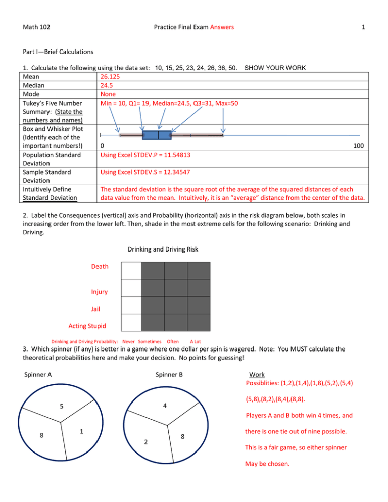
Math 102
Practice Final Exam Answers
1
Part I—Brief Calculations
1. Calculate the following using the data set: 10, 15, 25, 23, 24, 26, 36, 50. SHOW YOUR WORK
Mean
26.125
Median
24.5
Mode
None
Tukey’s Five Number
Min = 10, Q1= 19, Median=24.5, Q3=31, Max=50
Summary: (State the
numbers and names)
Box and Whisker Plot
(Identify each of the
important numbers!)
0
100
Population Standard
Using Excel STDEV.P = 11.54813
Deviation
Sample Standard
Using Excel STDEV.S = 12.34547
Deviation
Intuitively Define
The standard deviation is the square root of the average of the squared distances of each
Standard Deviation
data value from the mean. Intuitively, it is an “average” distance from the center of the data.
2. Label the Consequences (vertical) axis and Probability (horizontal) axis in the risk diagram below, both scales in
increasing order from the lower left. Then, shade in the most extreme cells for the following scenario: Drinking and
Driving.
Drinking and Driving Risk
Death
Injury
Jail
Acting Stupid
Drinking and Driving Probability: Never Sometimes
Often
A Lot
3. Which spinner (if any) is better in a game where one dollar per spin is wagered. Note: You MUST calculate the
theoretical probabilities here and make your decision. No points for guessing!
Spinner A
Spinner B
(5,8),(8,2),(8,4),(8,8).
4
5
Work
Possiblities: (1,2),(1,4),(1,8),(5,2),(5,4)
Players A and B both win 4 times, and
8
1
2
8
there is one tie out of nine possible.
This is a fair game, so either spinner
May be chosen.
Math 102
Practice Final Exam Answers
2
Part II. Use MS Excel to determine solutions to the following. Then copy the stated parts on this paper.
1. Are the scores on the data sheet for this problem normally
distributed?
Past histogram chart here
Frequency
Past Results of the 68-95-99% Rule:
12
Intervals
10
Min
68% 70.64588
95% 69.06176
99% 67.47764
Max
Actual % of Scores
73.81412
57
75.39824
100
76.98236
100
8
6
4
2
0
71
The data are NOT normally distributed. The 68-95-99% rule
fails and the histogram is neither centrally lumped nor
symmetrically skewed.
2. Researchers in a national study determined that 74% of
young people, ages 18-29 talk on handheld telephones while
driving. In a class of 32 students at CWU, 23 said they do the
same. Is the sample statistically like the population within a
95% confidence interval?
SD = √𝑛𝑝(1 − 𝑝) =SQRT(32*(.74)*(1-.74)) = 2.48
.74*32 = 23.68
3. A random sample of voters from Math 311 indicated the
voting choices shown in the data set. Based on 95% certainty,
is choice of a gubernatorial candidate dependent on choice of
a presidential candidate or not?
72
73
74
More
Show your Confidence Interval
(23.68-1.96*2.48, 23.68+1.96*2.48) = (18.8, 28.5)
State your Decision
The students at CWU are NOT significantly different
from the US population, because 23 is in the 95%
confidence interval above with the average for the US.
State your Chi-square value
Chi-square = 18. 6
Paste your 3-D Plot of Observed Values
State p-value
P = .0000165 which is much smaller than .05.
Presidential Choice vs Gubernatorial
Choice
16
20
10
1
6
0
O
R
I
M
Gubernatorial Choice
Count
Presidential
Choice
State your conclusion, based on comparing p with 5%
Reject Ho; Choice of presidential candidate is
significantly dependent on (or associated with) choice
of gupernatorial candidate (or vice versa.
Math 102
Practice Final Exam Answers
4. Suppose your probability of winning game is 1/3, and every Show your calculation here
time you win, you get $3. How much should you pay out if you
lose, so that the game is fair?
1/3*$3 = 2/3*X. Solve for X.
3
X = $1.50. In other words, you should pay $1.50 when
you lose, which is twice as probable as winning, but
when you win, you make twice as much as you lose!
That’s what makes this game fair in the long run.
5.
Suppose you take a road trip east from Ellensburg, setting your trip
meter to 0 at the beginning of the trip. Then at various times, you
note the mileage traveled and the time of travel. (See data sheet.)
What can you state about your average rate of speed by way of linear
regression.
Regression Equation
y = 57.89x - 10.99
Average speed
57.89 miles per hour
Paste Regression Chart
Accuracy of the Model
Time Enroute vs Distance
Traveled
R² = 0.9996
400
y = 57.89x - 10.988
R² = 0.9957
300
Distance 200
Traveled
(miles) 100
305
195
132
88
0
38
0
0
-100
265
1
2
3
4
Time Enroute (hours)
5
6