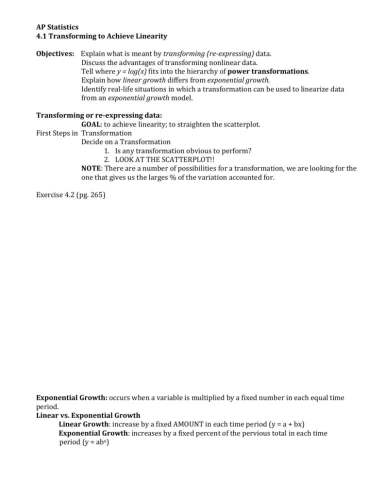
AP Statistics
4.1 Transforming to Achieve Linearity
Objectives: Explain what is meant by transforming (re-expressing) data.
Discuss the advantages of transforming nonlinear data.
Tell where y = log(x) fits into the hierarchy of power transformations.
Explain how linear growth differs from exponential growth.
Identify real-life situations in which a transformation can be used to linearize data
from an exponential growth model.
Transforming or re-expressing data:
GOAL: to achieve linearity; to straighten the scatterplot.
First Steps in Transformation
Decide on a Transformation
1. Is any transformation obvious to perform?
2. LOOK AT THE SCATTERPLOT!!
NOTE: There are a number of possibilities for a transformation, we are looking for the
one that gives us the larges % of the variation accounted for.
Exercise 4.2 (pg. 265)
Exponential Growth: occurs when a variable is multiplied by a fixed number in each equal time
period.
Linear vs. Exponential Growth
Linear Growth: increase by a fixed AMOUNT in each time period (y = a + bx)
Exponential Growth: increases by a fixed percent of the pervious total in each time
period (y = abx)
The Logarithm Transformation
 If the scatterplot of the data looks to be an exponential grow, try to map:
x  log y
 If the scatterplot of the data looks to be an exponential decay, try to map:
log x  y
 If you are dealing with the power model, try to map:
log x  log y
Algebraic Properties of Logarithms
logb x = y iff by = x
The rules of logarithms are
1. logb (MN) = logb M + logb N
𝑀
2. logb ( 𝑁 ) = logb M – logb N
3. lobb (x)p = p  logb x
NOTE: log is base 10 and ln is base “e” which is approximately 2.71828. For all transformations, you
can use either ln or the log.
Predictions
IMPORTANT NOTE: The transformed scatterplot and your LSRL models the transformed data and
you MUST reflect the transformation you employed (SHOW THE TRANSFORMATION IN YOUR LSR
EUATION!!!!)
Exponential Growth Model
Exercise 4.5 (pg.276)
Power Law Models
Exercise 4.11 (pg 285)
HW: pg. 288-291; 4.15, 4.16, 4.19, 4.21