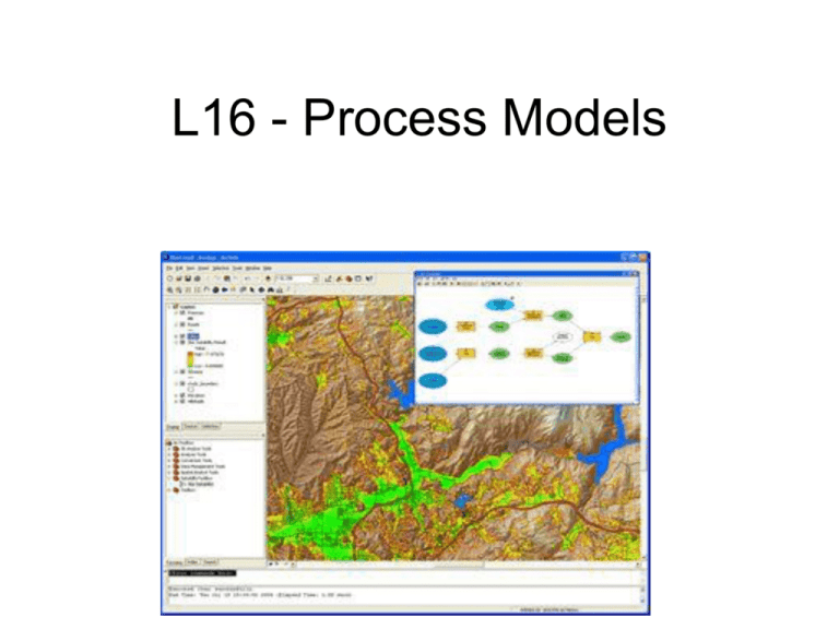
L16 - Process Models
Quick Review of Data
Models
Two major data models
– Vector
• Simple vector data structure
• Higher level data models
– TIN
– Dynamic segmentation
– Regions
– Raster (grid and image)
Representation Models
• Represent the objects of real
world through a sets of layers
(Data Models)
• Common data models/descriptive
models.
• Spatial relationships within an
object (the shape of a building).
• Between the other objects in the
landscape (the distribution of
buildings).
• Model the attributes of the objects
(who owns each building).
Process Models
• Describe the interaction
or processes of the
objects of real world,
which are modeled in the
representation model, by
using map calculation
•
•
•
•
Suitability modeling:
where should I put it?
Distance modeling:
how far is it?
Hydrologic modeling:
where will the water flow
to?
Surface modeling:
what is the pollution
level?
Why construct a process
model?
• We need to make decisions, and take
actions about spatial phenomenon.
• It may help us evaluate our understanding
of complex processes.
What type of model should we
construct?
Classification Schemes:
– Before (a priori) vs after (a posteriori) the fact.
– Natural and scale analog models
• Natural analog models uses real world objects or
events as the basis for the model.
• Scale analog models
– Mathematical models
• Deterministic
• Stochastic
may be either steady state or dynamic
• Optimization methods
– Conceptual models
Mathematical Models
• Static vs. dynamic: A dynamic model accounts for timedependent changes in the state of the system, while a
static (or steady-state) model calculates the system in
equilibrium, and thus is time-invariant. Dynamic models
typically are represented by differential equations.
• Deterministic vs. stochastic: A deterministic model is
one in which every set of variable states is uniquely
determined by parameters in the model and by sets of
previous states of these variables. Therefore,
deterministic models perform the same way for a given
set of initial conditions. Conversely, in a stochastic
model, randomness is present, and variable states are
not described by unique values, but rather by probability
distributions.
Mathematical Models
• Optimization Model: A model used to find the
best possible choice out of a set of alternatives.
It may use the mathematical expression of a
problem to maximize or minimize some function.
The alternatives are frequently restricted by
constraints on the values of the variables. A
simple example might be finding the most
efficient transport pattern to carry commodities
from the point of supply to the markets, given the
volumes of production and demand, together
with unit transport costs.
Global Mathematical Functions
Polynomial Trend Surface
Global Mathematical Functions
Kriged Surface
Creating a conceptual model to
solve a spatial problem (1)
• Step 1. Stating the problem.
– What is the goal?
• Step 2. Breaking the problem down.
– What are the objectives.
– What are the objects and their interactions
(process model).
– What datasets (data model and presentation
model) will be needed
Creating a conceptual model to
solve a spatial problem (2)
• Step 3. Exploring the datasets
– What is contained in the datasets
– what relationships between the datasets
• Step 4. Performing analysis (spatial analysis)
– Which tools to run the process models and build a
overall model
• Step 5. Verifying the model’s result
– Does any thing in the model need to be changed?
– If yes, go back to step 4
• Step 6. Implementing the result
Example using conceptual model to
create a suitability map
Step 1. Stating the problem
Step 2. Breaking the problem down
Process models
Datasets
(data models &
representation
model)
• Step 3. Exploring the datasets
Datasets
(data models &
representation
model)
Step 4. Performing analysis (spatial analysis)
Step 5. Verifying the model’s result
• to verify if the result is correct
Step 6. Implementing the result
• to building a new school in the chosen location
Process Modeling and GIS
• GIS uses:
– Natural and scale analog
– Conceptual and
– Mathematical modeling
• Either in isolation or combined in an
iterative process.
• Proprietary GIS software provides few if
any process models as part of the
standard set of functions – ArcGIS has
Model Builder
Modeling Physical and Environmental
Processes
• The following example comes from the
Department of Conservation: Bureau of
Geology, Natural Areas and Coastal
Resources
• http://www.maine.gov/doc/nrimc/mgs/expl
ore/hazards/landslide/facts/nov10.htm
Modeling Physical and Environmental
Processes
Figure 1. A clay bluff on the north shore of Rockland Harbor failed in 1996.
This landslide formed a new scarp about 200 feet landward of the original
top of the bluff in just a few hours. Two homes were destroyed as a result
of this catastrophic slide.
Figure 4. A large rotational slide occurred in
the spring of 2006 along Hobbs Brook in
Cumberland, Maine in an area of high relief
and steeply sloped stream bank. The slide
occurred after a heavy sustained rainfall.
Figure 5. In May of 2005 a landslide occurred in Wells along the banks
of the Merriland River. The slide destroyed a portion of a walking trail
in the Rachel Carson National Wildlife Refuge and removed the
backyard of a nearby house. Parts of the house's foundation were left
exposed and the house was declared unsafe to inhabit.
Figure 6. In May of 2006, a large earth flow caused by improper drainage due to
recent road construction occurred in Sanford, Maine. The drainage focused heavy
runoff towards this property, which then undercut the overlying sand, causing a large
earth flow into Branch Brook.
Figure 7. A landslide occurred along the Penobscot River in the town of Greenbush on
June 30, 2006. The slide undercut Route 2 and caused this section of roadway to be
closed until the river bank stabilized, and the roadway section was rebuilt.
Risk Factor Analysis
• The Landslide Susceptibility Maps were created using Risk Factor
Analysis based on the following principles:
– It is likely that landslides will occur where they have occurred in the
past.
– Landslides are likely to occur in similar geological, geomorphological,
and hydrological conditions as they have in the past.
• Simply put:
– All available data is collected for risk factors that are located within the
area of study.
– Next, all landslide locations within this same area are systematically
mapped.
– Using a Geographic Information System (GIS), mapped landslides are
compared to each risk factor and examined to determine which risk
factors are the most statistically significant causes of landslides.
– Once the analysis is complete, statistically significant risk factors are
mapped, and zones of landslide susceptibility are created, ranging from
areas of no risk factors (lowest landslide potential) to areas where there
are 3 or more risk factors present (highest landslide potential).
Landslide Risk Factors
Risk Factors Used in This Study
• Geomorphic Risk Factors
– Slope: The steeper the slope, the larger the shear stress on the
materials and the more susceptible the slope is to failure
– Curvature (concave): Concave topography will concentrate groundwater
flow, raising pore pressures and reducing shear strength of the soil.
– Slope aspect: Repeated freeze/thaw cycles reduce the shear strength of
the shallow soil material, increasing the likelihood of shallow soil slumps
and creep.
– Relief/slope height: As the thickness of the potential landslide block
increases, the shear stress on the lower section of block increases,
making the block (slope) more susceptible to failure. Therefore, thicker
sections of surficial materials will be more susceptible to landslides.
• Soil properties
– Surficial geologic materials: Cohesive materials such as clays are prone
to landslides along planes of weakness in the sediment. Less cohesive
materials (sands) may slump if slopes oversteepen or ground water
pore pressure increases and reduces internal friction.
Figure 8
Figure 9
Figure 10
Figure 11
Figure 12
Figure 13
Figure 14
Figure 15
Figure 16
Figure 17
Limitations of the maps
• Town-level landslide mapping is required to validate
the susceptibility maps and provide credibility to local
and State officials.
• Landslide susceptibility maps indicate where
landslides are likely to occur, not whether or when a
landslide will occur.
• The maps are based on landslide sites mapped below
the glacial marine limit. Extension to other geologic
settings would require additional study.
– 18% of landslides occur on glacial till
• Additional statistical analysis and incorporation of
additional risk factors may improve the usefulness of
the susceptibility maps. Data for additional risk factors
must be available throughout the study area.
Applicability of the maps
• The maps identify where landslides have
already occurred and where future
landslides may occur.
• Public education.
• The effects of future landslides may be
mitigated by adopting appropriate building
codes or land use policies in landslide
prone areas.
Conclusions
• Utilizing input and reviews of maps from local
and state officials will enhance future map
products.
• Acquisition of LIDAR data will enhance
quality and accuracy of maps.
• Updating Maine's landslide inventory
database will increase the accuracy and
utilization of the maps.
• Landslide susceptibility mapping is an
ongoing process and will continually evolve
into a more useful tool for landslide hazard
mitigation.
Modeling Human Processes
• It is difficult to model humans spatial
behavior.
– How do people move through space when
constrained by roads, buildings, fences, etc.?
– How do people choose where to live, shop,
vacation?
Spatial Interaction Models
• An abstract, idealized, representation of any and
all kinds of spatial interaction phenomenon.
• It is the flow of products, people, services, or
information among places, in response to
localized supply and demand.
• These models describe the flows between a set
of origin and destination zones on a map.
• These are commercial models outside of most
GIS packages.
Three interdependent conditions are necessary
for a spatial interaction to occur:
– Complementarity. There must be a supply and a
demand between the interacting locations; e.g., a
store and its customers.
– Intervening opportunity. There must not be another
location that may offer a better alternative as a point
of origin or as a point of destination. For instance, in
order to have an interaction of a customer to a store,
there must not be a closer store that offers a similar
array of goods.
– Transferability. Freight, persons or information being
transferred must be supported by transport
infrastructures, implying that the origin and the
destination must be linked.
Inputs and Outputs
Origin Totals
Destination
Totals
Interzonal
Costs
Spatial Interaction Model
(an equation)
Predicted Trips
Beta
Deterrence
Parameter
Origin/Destination Matrix
http://people.hofstra.edu/geotrans/
eng/methods/odmatrix.html
The Relationship between Distance
and Interaction
The above figure portrays a classic non-linear relationship between distance and
the level of interactions of location A with other locations (B, C and D). It assumes
that each location has the same complementarity level and that no intervening
opportunities are present. The closest location, B, has the highest level of
interaction with location A, while locations C and D have lower levels of interaction
since they are located further away.
http://people.hofstra.edu/geotrans/
eng/methods/distancedecay.html
Three Basic Interaction Models
http://people.hofstra.edu/geotrans/
eng/methods/threebasicmodels.ht
Three Basic Interaction Models
1. Gravity model. The level of
interaction between two
locations is measured by
multiplying their attributes,
which is then pondered by
their level of separation.
Separation is often squared to
reflect the growing friction of
distance. On the above figure,
two locations (i and j) have a
respective "weight"
(importance) of 35 and 20 and
are at a distance (degree of
separation) of 8. The resulting
interaction is 10.9, which is
reciprocal.
http://people.hofstra.edu/geotrans/
eng/methods/threebasicmodels.ht
Three Basic Interaction Models
2. Potential model. The level of
interaction between one
location and all the others is
measured by the summation of
the attributes of each other
location pondered by their
level of separation (again
squared to reflect the friction of
distance). On the above figure,
the potential interaction of
location i (Ti) is measured by
adding the ratio "weight" /
squared distance for each
other locations (j, k and l). The
potential interaction is 3.8,
which is not reciprocal.
http://people.hofstra.edu/geotrans/
eng/methods/threebasicmodels.ht
Three Basic Interaction Models
3. Retail model. This model
deals with boundaries, instead
of interactions. It assumes that
the market boundary between
two locations is a function of
their separation pondered by
the ratio of their respective
weights. If two locations have
the same importance, their
market boundary would be
halfway between. On the
above figure, the market
boundary between locations i
and j (Bij) is at a distance of
4.9 from i (and consequently at
a distance of 2.1 from j).
http://people.hofstra.edu/geotrans/
eng/methods/threebasicmodels.ht
Conventional Models
Are:
– Over 25 years old.
– Reflect a data poor era.
– Non-linear but only in a simple way.
– Designed to minimize computation.
– Possibly poor performer.
Neural Networks
• Make use of AI.
• Uses data to learn (or discover) patterns
and relationships instead of relying totally
on people to specify them.
• It offers equation free modeling.
• It is highly automated modeling.
• It has universal modeling capabilities
• It is noisy data resistant.
Modeling the Decision Making
Process
• Outputs from process models are the raw
information required for making decisions.
• Map overlay is the traditional method for spatial
decision making, however this can be
problematic:
– Overlay can be difficult to understand if multiple
factors are involved.
– Some GIS packages do not allow different weights for
the variables.
– Threshold values, important for polygon overlay, may
be based on opinion.
The Solution
• Use Multi-Criteria Evaluation (MCE)
Techniques.
• This allows map layers to be weighted,
based on importance.
• This also has problems:
– Different algorithms produce slightly different
results.
– The specification of weights is also based on
opinion.