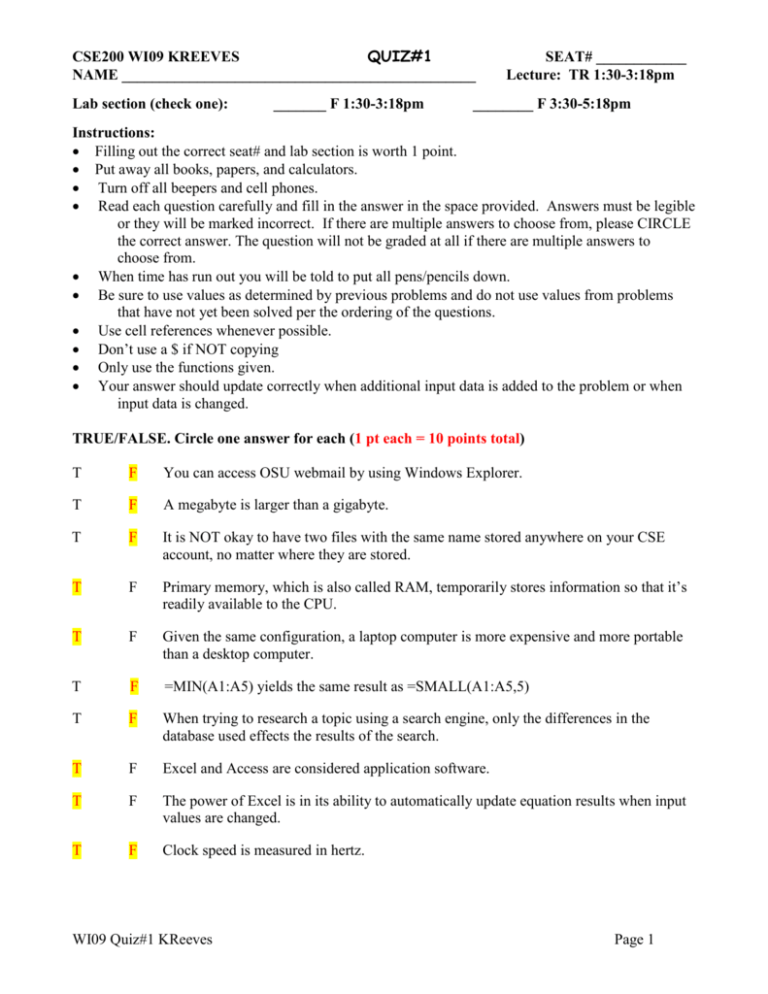
CSE200 WI09 KREEVES
QUIZ#1
NAME _______________________________________________
Lab section (check one):
_______ F 1:30-3:18pm
SEAT# ____________
Lecture: TR 1:30-3:18pm
________ F 3:30-5:18pm
Instructions:
 Filling out the correct seat# and lab section is worth 1 point.
 Put away all books, papers, and calculators.
 Turn off all beepers and cell phones.
 Read each question carefully and fill in the answer in the space provided. Answers must be legible
or they will be marked incorrect. If there are multiple answers to choose from, please CIRCLE
the correct answer. The question will not be graded at all if there are multiple answers to
choose from.
 When time has run out you will be told to put all pens/pencils down.
 Be sure to use values as determined by previous problems and do not use values from problems
that have not yet been solved per the ordering of the questions.
 Use cell references whenever possible.
 Don’t use a $ if NOT copying
 Only use the functions given.
 Your answer should update correctly when additional input data is added to the problem or when
input data is changed.
TRUE/FALSE. Circle one answer for each (1 pt each = 10 points total)
T
F
You can access OSU webmail by using Windows Explorer.
T
F
A megabyte is larger than a gigabyte.
T
F
It is NOT okay to have two files with the same name stored anywhere on your CSE
account, no matter where they are stored.
T
F
Primary memory, which is also called RAM, temporarily stores information so that it’s
readily available to the CPU.
T
F
Given the same configuration, a laptop computer is more expensive and more portable
than a desktop computer.
T
F
=MIN(A1:A5) yields the same result as =SMALL(A1:A5,5)
T
F
When trying to research a topic using a search engine, only the differences in the
database used effects the results of the search.
T
F
Excel and Access are considered application software.
T
F
The power of Excel is in its ability to automatically update equation results when input
values are changed.
T
F
Clock speed is measured in hertz.
WI09 Quiz#1 KReeves
Page 1
A
1
2
3
4
5
6
7
8
9
10
11
12
B
C
EXCEL-LENT ICE CREAM PARLOR
D
E
F
G
H
I
J
K
cone type
price ==> $1.00 $1.00 $1.50 $2.00
cost
scoops sugar waffle bowl scoops sugar waffle bowl total
name
type
raspberry chip
ice cream
3
0
0
1
$3.00 $0.00 $0.00 $2.00 $5.00
cookies and cream
ice cream
1
1
0
0
$1.00 $1.00 $0.00 $0.00 $2.00
choc chip cookie dough ice cream
2
0
1
0
$2.00 $0.00 $1.50 $0.00 $3.50
vanilla bean
frozen yogurt
1
1
0
0
$1.00 $1.00 $0.00 $0.00 $2.00
strawberry
sorbet
2
0
1
0
$2.00 $0.00 $1.50 $0.00 $3.50
choc fudge brownie
ice cream
2
0
0
1
$2.00 $0.00 $0.00 $2.00 $4.00
black cherry swirl
frozen yogurt
1
1
0
0
$1.00 $1.00 $0.00 $0.00 $2.00
mango peach
sorbet
3
0
0
1
$3.00 $0.00 $0.00 $2.00 $5.00
what percent of people want each cone type?
38% 25% 38%
FUNCTIONS
AVERAGE(number1,number2,…)
COUNT(number1,number2,…)
LARGE(array,k)
MAX(number1,number2,…)
MIN(number1,number2,…)
RANK( number, ref, order)
ROUND(number, num_digits)
SMALL(array,k)
SUM(number1,number2,…)
1. (6 pts) Evaluate the following functions in two ways. The first way is to evaluate exactly as you see the data
in the worksheet given above. The second way is to delete all the zeroes in the range E4:E11; that is, instead of
the zeroes in E4:E11, there is a blank value instead.
as shown above
if blanks instead of zeroes
=COUNT(E4:E11)
_____8_____
____2______
=AVERAGE(E4:E11)
_____0.25__
____1______
=MIN(E4:E11)
_____0_____
____1______
2. ( 7 pts) Write an Excel formula in cell D12, which can be copied across to cell F12, to determine the
percent of people who ordered a “sugar” cone type. NOTE: Remember that the wording of this problem refers to
the determining of the percent of people who ordered “waffle” then “bowl” cone types as the equation you give
as a solution is copied across.
=SUM(D4:D11)/COUNT(D4:D11)
Okay if used columns C, E or F on the count function; $ okay on the column as well
=SUM(D4:D11)/SUM($D4:$F11)
=AVERAGE(D4:D11)
Accepted countif(d4:d11,1) or criteria variation of “1”, “=1”, “>0”, “<>0”
Optional $ on row
b. (5 pts) Write an Excel formula in cell D13 (not shown), which can be copied across to cell F13, to round
the percent given in the above problem to the nearest tenth of a percent.
=ROUND(D12,3)
Optional $ on row
3. (5 pts) If I enter the formula =D12+E12+F12, Excel returns 100%, however, if I add up the values as shown
in the worksheet by hand, the values add up to 101%. Explain how the 100% value was obtained and how the
101% value was obtained.
101% because that’s what the FORMATTED/DISPLAYED values add up to but
100% because that’s the correct PRECISE/ACTUAL value
4. (7 pts) Write an Excel formula in cell G4, which can be copied down and across to cell J11, to determine the
cost ice cream scoops specified for the raspberry chip order. NOTE: Remember that the wording of this problem
refers to determining the cost of scoops for each flavor as well as the cost of each cone type using the equation
you give as a solution since this is a copy down and across problem.
=C4*C$2
WI09 Quiz#1 KReeves
Page 2
No extra $ signs allowed
5. (5 pts) Write an Excel formula in cell K4, which can be copied down to cell K11, to determine the total cost
of the raspberry chip order i.e. scoop cost plus cone cost. NOTE: Be sure to give an answer that will
automatically update should further costs to be added to the order. For instance, if I add another type of cone
between columns G and H, a flavored topping, or whipped cream, your solution should still work.
=SUM(G4:J4)
Optional $ on column
6. (4 pts) I put the formula =RANK(K4,K$4:K$11,1) in cell L4. Determine the results of this formula
assuming it’s copied down to cell L11.
L
4
7
5
1
6
4
7
1
8
4
9
6
10
1
11
7
SCORE _____________/50
WI09 Quiz#1 KReeves
Page 3