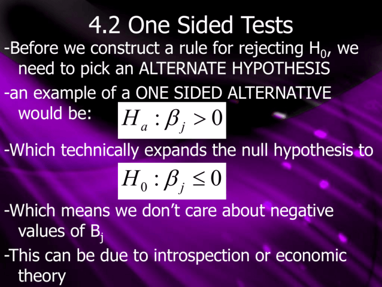
4.2 One Sided Tests
-Before we construct a rule for rejecting H0, we
need to pick an ALTERNATE HYPOTHESIS
-an example of a ONE SIDED ALTERNATIVE
would be:
H : 0
a
j
-Which technically expands the null hypothesis to
H0 :  j  0
-Which means we don’t care about negative
values of Bj
-This can be due to introspection or economic
theory
4.2 One Sided Tests
-If we pick an α (level of significance) of 5%, we
are willing to reject H0 when it is true 5% of
the time
-in order to reject H0, we need a “sufficiently
large” positive t value
-a one sided test with α=0.05 would leave 5% in
the right tail with n-k-1 degrees of freedom
-our rejection rule becomes reject H0 if:
t ˆ  t *
j
-where t* is our CRITICAL VALUE
4.2 One Sided Example
-Take the following regression where we are
interested in testing whether Pepsi
consumption has a +’ve effect on coolness:
Coˆol  4.3 0.3 Geek  0.5 Pepsi
2.1
R  0.62
2
0.25
0.21
N  43
-We therefore have the following hypotheses:
H0 : 2  0
H a : 2  0
4.2 One Sided Example
-We then construct our test statistic:
ˆ

t ˆ  2
2
0.5


2
.
38
0.21
se( ˆ2 )
-With degrees of freedom=43-3=40 and a 1%
significance level, from a t table we find that
our critical t, t*=2.423
-We therefore do not reject H0 at a 1% level of
significance; Pepsi has no positive effect on
coolness at the 1% significance level in our
study
4.2 One Sided Tests
-From looking at a t table, we see that as
the significance level falls, t* increases
-We therefore need a bigger test t statistic
in order to reject H0 (the hypothesis that a
variable is not significant)
-as degrees of freedom increase, the t
distribution approximates the normal
distribution
-after df=120, one can in practice use
normal critical values
4.2 One Sided Tests
-The other one-sided test we can conduct is:
Ha :  j  0
-Which technically expands the null hypothesis to
H0 :  j  0
-Here we don’t care about positive values of Bj
-We now reject H0 if:
t ˆ  t *
j
4.2 Two Sided Tests
-It is important to decide the nature of our onesided test BEFORE running our regression
-It would be improper to base our alternative on
whether Bjhat is positive or negative
-A way to avoid this and a more general test is a
two-tailed (or two sided) test
-Two sided tests work well when a variable’s sign
isn’t determined by theory or common sense
-Our alternate hypothesis now becomes:
Ha :  j  0
4.2 Two Sided Tests
-For a two sided test, we reject H0 if:
| t | t *
-In finding our t*, since we now have two
rejection regions, α/2 will fit into each tail
-For example, if α=0.05, we will have 2.5% in
each tail
-When we reject H0, we say that “xj is statistically
significant at the ()% level”
-When we do not reject H0, we say that “xj is
statistically insignificant at the ()% level”
4.2 Two Sided Example
-Going back to our Pepsi example, we instead ask
if Pepsi has ANY effect (positive or negative) on
coolness:
Coˆol  4.3 0.3 Geek  0.5 Pepsi
2.1
R  0.62
2
0.25
0.21
N  43
-We therefore have the following hypotheses:
H0 : 2  0
H a : 2  0
4.2 Two Sided Example
-We then construct our same test statistic as
before:
ˆ

t ˆ  2
2
0.5


2
.
38
0.21
se( ˆ2 )
-With degrees of freedom=43-3=40 and a 1%
significance level, from a t table we find that
our critical t, t*=2.704 (bigger than before)
-We therefore reject H0 at a 1% level of
significance; Pepsi has an effect on coolness at
the 1% significance level in our study
4.2 Other Simple Tests
-We sometimes want to test whether Bj is equal
to a certain number, such as:
H0 :  j  a j
-Which makes the alternate hypothesis:
Ha :  j  a j
-Which changes our test t statistic to (t* is found
the same from tables):
ˆ j  a j
(estimate - hypothesis value)
t

standard error
se( ˆ j )
4.2 Another Pepsi Example
-Foolishly, we forget that coolness is a log-log
model (see GH 2009), making each slope
parameter the partial elasticity:
ln( Coˆol )  1.7 0.2 ln( Geek )  0.7 ln( Pepsi)
0.4
R  0.71
2
0.15
0.28
N  43
-wanting to see if Pepsi has a unit partial
elasticity, we have the following hypotheses:
H0 : 2  1
H a : 2  1
4.2 Two Sided Example
-We then construct our new test statistic:
t ˆ 
2
ˆ2  a j
0.7  1



1
.
07
0.28
se( ˆ2 )
-With degrees of freedom=43-3=40 and a 1%
significance level, from a t table we find that
our critical t, t*=2.704 (same as 2-tailed)
-Therefore don’t reject H0 at a 1% level of
significance; Pepsi may have unit partial
elasticity at the 1% significance level
4.2 p-values
-So far we have taken a CLASSICAL approach to
hypothesis tests
-choosing an α ahead of time can skew our
results
-if a variable is insignificant at 1%, but
significant at 5%, it is still highly significant!
-we can instead ask: “given the observed value of
the t statistic, what is the SMALLEST significance
level at which the null hypothesis would be
rejected? This level is known as the P-VALUE.”
4.2 p-values
-P-VALUES relate to probabilities and are
therefore always between zero and 1
-regression packages (such as Shazam)
usually report p-values for the null
hypothesis Bj=0
-testing commands can give other p-values
of the form:
P (| t || t* |)
-ie: P-values are the areas in the tails
4.2 p-values
-a small p-value argues for rejecting the null
hypothesis
-a large p-value argues for not rejecting the null
hypothesis
-once a level of significance (α) has been chosen,
reject H0 if:
P 
-regression packages generally list the p-value for
a two-tailed test.
-for a one-tailed test, simply use p/2
4.2 Statistical Mumbo-Jumbo
-If we reject H0, we can state that “Ho is rejected
at a ()% level of significance’
-If we do not reject H0, we CANNOT say that “H0
is accepted at a ()% level of significance”
-while a null hypothesis of H0:Bj=2 may be not
rejected, a similar H0:Bj=2.2 may also not be
rejected
-Bj cannot equal both 2 and 2.2
-we can conclude a certain number ISN’T valid,
but we can’t conclude on ONE valid number
4.2 Economic and Statistical Significance
-STATISTICAL significance depends on the value
of t
-ECONOMIC significance depends upon the size
of Bj
-since we know that t depends on the size and
standard error of Bj:
ˆ j
t ˆ 
j
se( ˆ )
j
-a coefficient may test significant due to a very
small se(Bj); a STATISTICALLY significant
coefficient may be too small to be
economically significant
4.2 Insignificant Example
-Theoretically, World Peace (WP) can only be
achieved if House (H) episodes resume and
people eat more chicken (C):
WPˆ   2.4 0.1 House  0.00045 Chicken
(1.7 )
( 0.01)
( 0.000071)
-although both House and Chicken would test as
being significant variables (their standard errors
are very small compared to their values), B3 is
so small chicken has a very small impact
-you’d have to eat so much chicken to cause
world peace it’s ECONOMICALLY insignificant
4.2 Significance and Large Samples
-As sample size increases, standard errors also
tend to increase
-coefficients tend to be more statistically
significant in large samples
-some researchers argue for smaller
significance levels in large samples and larger
significance levels in small samples
-this can often be due to an agenda
-in large samples, it is important to examine the
MAGNITUDE of any statistically significant
variables.
4.2 Multicollinearity Strikes Back
-Recall that large standard errors can also
be caused by Multicollinearity
-This can cause small t stats and
insignificance
-This can be fought by
1) Collecting more data
2) Dropping or combining (preferred)
independent variables
4.2 3 Easy (honest) steps for tests
When testing, follow these 3 easy steps:
1) If a variable is significant, examine its
coefficient’s magnitude and explain its
impact (this may be complicated if not
linear)
2) If a variable is insignificant at usual
levels, check it’s p-value to see if some
case for significance can be made
3) If a variable has the “wrong” sign, ask
why – are there omitted variables or
other issues?