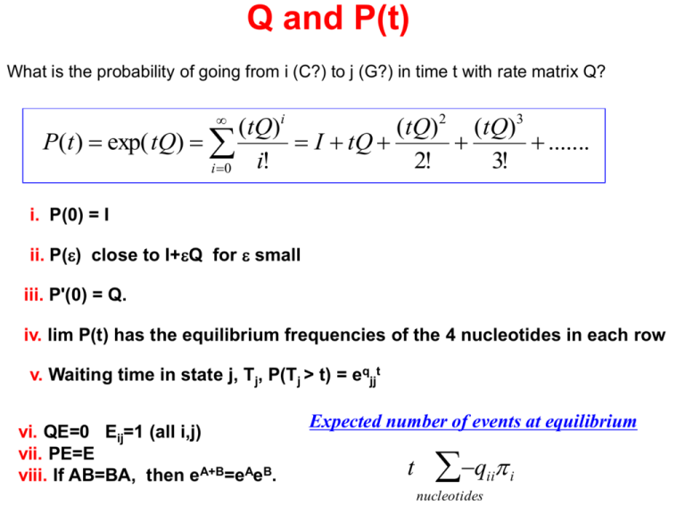
Q and P(t)
What is the probability of going from i (C?) to j (G?) in time t with rate matrix Q?

(tQ)i
(tQ)2 (tQ)3
P(t )  exp( tQ)  
 I  tQ 

 .......
i!
2!
3!
i 0
i. P(0) = I
ii. P(e) close to I+eQ for e small
iii. P'(0) = Q.
iv. lim P(t) has the equilibrium frequencies of the 4 nucleotides in each row
v. Waiting time in state j, Tj, P(Tj > t) = eqjjt
vi. QE=0 Eij=1 (all i,j)
vii. PE=E
viii. If AB=BA, then eA+B=eAeB.
Expected number of events at equilibrium
t
q 
ii
nucleotides
i
Jukes-Cantor (JC69): Total Symmetry
Rate-matrix, R:
T
A
F
R
O
M
C
O
G
T
3*a
a
a
a
a
3*a
a
a
aa3*aa
aaa3*a
A
C
G
T
Transition prob. after time t, a = a*t:
P(equal) = ¼(1 + 3e-4*a ) ~ 1 - 3a
P(diff.) = ¼(1 - 3e-4*a ) ~ 3a
Stationary Distribution: (1,1,1,1)/4.
5
1
P  P( s1)  P( s1i  s2i )  ( )5 P(T  T)P(C  G)P(G  G)P(G  T)P(A  T)
i 1
4
1 1
 ( )5 ( )5 (1  3e 4 a )2 (1  e 4 a )3
4 4
Principle of Inference: Likelihood
Likelihood function L() – the probability of data as function of parameters: L(Q,D)
LogLikelihood Function – l(): ln(L(Q,D))
If the data is a series of independent experiments L() will become a product of Likelihoods of
each experiment, l() will become the sum of LogLikelihoods of each experiment
ˆ (D)  Q as data increases.
Consistenc y : Q
true
Likelihood
LogLikelihood
In Likelihood analysis parameter is not viewed as a random variable.
From Q to P for Jukes-Cantor
 3a
 a

 a

 a
a
a
a 
1
1
 3 1
 1 3 1
 3a
a
a 
1
 a

a
 3a
a 
1 3 1 
1



a
a
 3a 
1
1  3
1
3a a
 
a 3a

 a a
i 0

a
 a
3 1

1 3

1/4[I 
1 1

1 1
i
1
1
1
1
 3 1
 3 1
 1 3 1
 1 3 1
1
1
i

1

 4 

1 3 1 
1 3 1 
1
1




1
1  3
1
1  3
1
1
i
3 1 1 1 
a
a 




a
a  i
1
3
1
1
/i!] 
t /i! 1/4[I   (4at) i 
1 1 3 1 
3a a 
i1



a 3a 
1
1
1
3


1 1

1 1 4 at
e ]
3 1

1 3 
Exponentiation/Powering of Matrices
1 0

0 2
1

If Q  BB where  
0 0

0 0
0 

0 0 
then Qi  BB1BB1...BB1  Bi B1
3 0 

0 4 
exp t1
0
0
0 






i
1 i
i
0
exp
t

0
0
(tQ)
(tBB )
(t) 1
2
B1

 B[
]B  B
and 
 0
0
exp t3
0 
i! i 0
i!
i!
i 0
i 0


0
0
exp t4 
 0
By eigen values:
0
Finding : det (Q-I)=0
JC69:
Finding B: (Q-iI)bi=0
1 1/4
1/4 1/4 1/4 1/4 
0 1 1
0
0
0




1
1/4
0
1
0
exp
4t
a
0
0
1/8
1/8
1/8
1/8



P(t)  
1 1/4 1 0 0
 0
0
exp 4ta
0
0
1
1 




0
0
exp 4ta  1
1
0
0 
1 1/4 1 0 0

Numerically:

k
(tQ) i
(tQ) i
 i! ~  i!
i 0
i 0
where k ~6-10
Kimura 2-parameter model - K80
TO
A
C
G
T
F A
-2*babab
R C
b2*baba
Q: O
G
M T
a = a*t
ab2*bab
bab2*ba
b = b*t
P(t)
start
.25(1  e4b  2e2( a b) )
.25(1  e4b )
.25(1  e4b  2e2( a b ) )
.25(1  e4b )
Felsenstein81 & Hasegawa, Kishino & Yano 85
Unequal base composition:
Qi,j = C*πj
(Felsenstein, 1981 F81)
i unequal j
Rates to frequent nucleotides are high - (π =(πA , πC , πG , πT)
Tv/Tr = (πT πC +πA πG )/[(πT+πC )(πA+ πG )]
A
T
C
G
Tv/Tr & compostion bias (Hasegawa, Kishino & Yano, 1985 HKY85)
(a/b)*C*πj
Qi,j =
C*πj
i- >j a transition
i- >j a transversion
Tv/Tr = (a/b) (πT πC +πA πG )/[(πT+πC )(πA+ πG )]
Measuring Selection
ThrSer
ACGTCA
ThrPro
ACGCCA
Certain events have functional
consequences and will be selected
out. The strength and localization of
this selection is of great interest.
-
ThrSer
ACGCCG
ArgSer
AGGCCG
The selection criteria could in
principle be anything, but the
selection against amino acid changes
is without comparison the most
important
ThrSer
ACTCTG
AlaSer
GCTCTG
AlaSer
GCACTG
The Genetic Code
3 classes of sites:
4
2-2
1-1-1-1
i.
4 (3rd)
Problems:
1-1-1-1 (3rd)
ii. TA (2nd)
i. Not all fit into those categories.
ii. Change in on site can change the status of another.
Possible events if the genetic code
remade from Li,1997
Possible number of substitutions: 61 (codons)*3 (positions)*3 (alternative nucleotides).
Substitutions
Number
Percent
Total in all codons
549
100
Synonymous
134
25
415
75
Missense
392
71
Nonsense
23
4
Nonsynonymous
Kimura’s 2 parameter model & Li’s Model.
Probabilities:
Rates:
start
b
.25(1  e4b  2e2( a b) )
b
a
b
.25(1  e4b )
a
.25(1  e4b  2e2( a b ) )
.25(1  e4b )
Selection on the 3 kinds of sites (a,b)(?,?)
1-1-1-1
(f*a,f*b)
2-2
(a,f*b)
4
(a, b)
alpha-globin from rabbit and mouse.
Ser
TCA
*
TCG
Ser
Sites
1-1-1-1
2-2
4
Thr
ACT
*
ACA
Thr
Glu
GAG
*
GGG
Gly
Total
274
77
78
Z(at,bt) = .50[1+exp(-2at) - 2exp(-t(a+b)]
Y(at,bt) = .25[1-exp(-2bt )]
X(at,bt) = .25[1+exp(-2at) + 2exp(-t(ab)]
Met
ATG
*
ATA
Ile
Cys
TGT
*
TAT
Tyr
Leu
TTA
*
CTA
Leu
Met Gly Gly
ATG GGG GGA
* **
ATG GGT ATA
Met Gly Ile
Conserved
246 (.8978)
51 (.6623)
47 (.6026)
Transitions
12(.0438)
21(.2727)
16(.2051)
Transversions
16(.0584)
5(.0649)
15(.1923)
transition
transversion
identity
L(observations,a,b,f)=
C(429,274,77,78)* {X(a*f,b*f)246*Y(a*f,b*f)12*Z(a*f,b*f)16}* {X(a,b*f)51*Y(a,b*f)21*Z(a,b*f)5}*{X(a,b)47*Y(a,b)16*Z(a,b)15}
where a = at and b = bt.
Estimated Parameters:
1-1-1-1
2-2
4
a = 0.3003 b = 0.1871
Transitions
a*f = 0.0500
a
= 0.3004
a
= 0.3004
2*b = 0.3742 (a + 2*b) = 0.6745 f = 0.1663
Transversions
2*b*f = 0.0622
2*b*f = 0.0622
2*b
= 0.3741
Expected number of:
replacement substitutions 35.49
synonymous
Replacement sites : 246 + (0.3742/0.6744)*77 = 314.72
Silent sites
: 429 - 314.72
= 114.28
Ks = .6644 Ka = .1127
75.93
Extension to Overlapping Regions
Hein & Stoevlbaek, 95
1st
1-1-1-1
2-2
1-1-1-1 sites
(f1f2a, f1f2b)
(f2a, f1f2b)
(f2a, f2b)
2-2
(f1a, f1f2b)
(f2a, f1f2b)
(a, f2b)
4
(f1a, f1b)
(a, f1b)
(a, b)
2nd
4
pol
gag
Example: Gag & Pol from HIV
Pol
Gag
1-1-1-1
2-2
4
1-1-1-1 sites
64
31
34
2-2
40
7
0
4
27
2
0
MLE:
a=.084
b= .024
a+2b=.133
fgag=.403
fpol=.229
Ziheng Yang has an alternative model to this, were sites are lumped into the same category if they have the same configuration of positions and reading frames.
HIV1 Analysis
Hasegawa, Kisino & Yano Subsitution Model Parameters:
a*t
0.350
0.015
A
0.361
0.004
β*t
0.105
0.005
C
0.181
0.003
G
0.236
0.003
Selection Factors
GAG
POL
VIF
VPR
TAT
REV
VPU
ENV
NEF
0.385
0.220
0.407
0.494
1.229
0.596
0.902
0.889
0.928
(s.d.
(s.d.
(s.d.
(s.d.
(s.d.
(s.d.
(s.d.
(s.d.
(s.d.
0.030)
0.017)
0.035)
0.044)
0.104)
0.052)
0.079)
0.051)
0.073)
Estimated Distance per Site: 0.194
0.222
T
Statistical Test of Models
(Goldman,1990)
Data: 3 sequences of length L
ACGTTGCAA ...
AGCTTTTGA ...
TCGTTTCGA ...
A. Likelihood (free multinominal model 63 free parameters)
L1 = pAAA#AAA*...pAAC#AAC*...*pTTT#TTT where pN1N2N3 = #(N1N2N3)/L
B. Jukes-Cantor and unknown branch lengths
ACGTTGCAA ...
l1
l2
l3
TCGTTTCGA ...
L2 = pAAA(l1',l2',l3') #AAA*...*pTTT(l1',l2',l3') #TTT
AGCTTTTGA ...
Test statistics: I. S (expected-observed)2/expected or II: -2 lnQ = 2(lnL1 - lnL2)
JC69 Jukes-Cantor: 3 parameters => c2 60 d.of freedom
Problems: i. To few observations pr. pattern.
Parametric bootstrap:
i. Maximum likelihood to estimate the parameters.
iii. Make simulated distribution of -2 lnQ.
ii. Many competing hypothesis.
ii. Simulate with estimated model.
iv. Where is real -2 lnQ in this distribution?
Rate variation between sites:iid each site
The rate at each position is drawn independently from a distribution, typically a G (or
lognormal) distribution. G(a,b) has density xb-1*e-ax/G(b) , where a is called scale
parameter and b form parameter.
Let L(pi,Q,t) be the likelihood for observing the i'th pattern, t all time lengths, Q the
parameters describing the process parameters and f (ri) the continuous distribution of
rate(s). Then L 
L( p , Q, r ) f ( r )dr

i
i
i
i