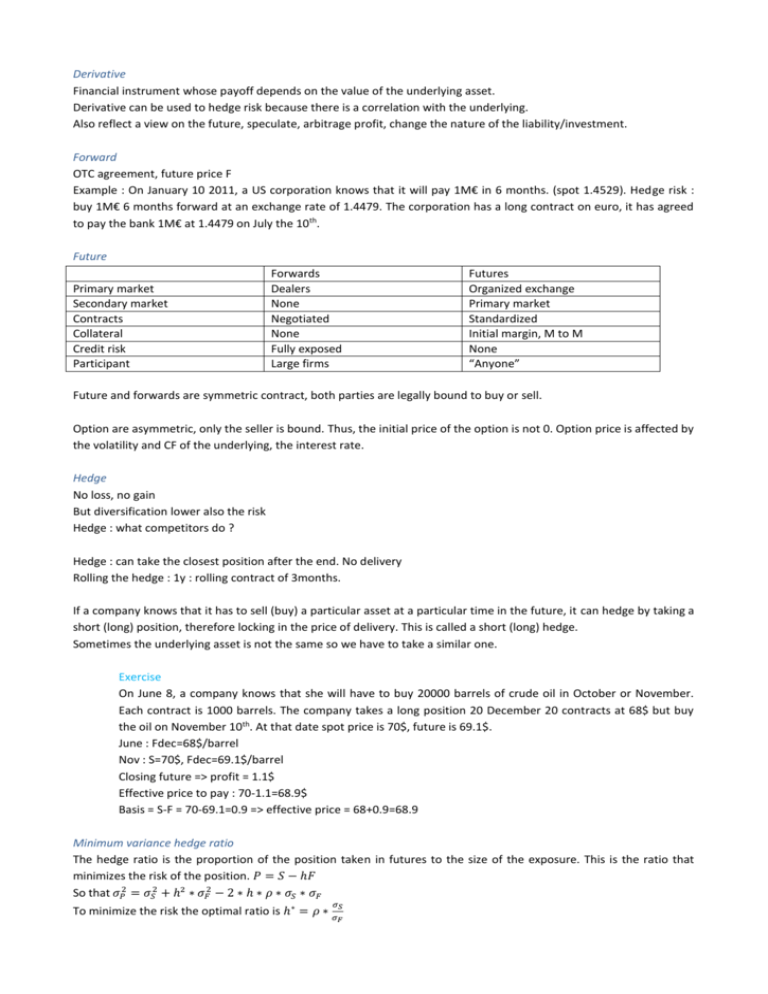
Derivative
Financial instrument whose payoff depends on the value of the underlying asset.
Derivative can be used to hedge risk because there is a correlation with the underlying.
Also reflect a view on the future, speculate, arbitrage profit, change the nature of the liability/investment.
Forward
OTC agreement, future price F
Example : On January 10 2011, a US corporation knows that it will pay 1M€ in 6 months. (spot 1.4529). Hedge risk :
buy 1M€ 6 months forward at an exchange rate of 1.4479. The corporation has a long contract on euro, it has agreed
to pay the bank 1M€ at 1.4479 on July the 10th.
Future
Primary market
Secondary market
Contracts
Collateral
Credit risk
Participant
Forwards
Dealers
None
Negotiated
None
Fully exposed
Large firms
Futures
Organized exchange
Primary market
Standardized
Initial margin, M to M
None
“Anyone”
Future and forwards are symmetric contract, both parties are legally bound to buy or sell.
Option are asymmetric, only the seller is bound. Thus, the initial price of the option is not 0. Option price is affected by
the volatility and CF of the underlying, the interest rate.
Hedge
No loss, no gain
But diversification lower also the risk
Hedge : what competitors do ?
Hedge : can take the closest position after the end. No delivery
Rolling the hedge : 1y : rolling contract of 3months.
If a company knows that it has to sell (buy) a particular asset at a particular time in the future, it can hedge by taking a
short (long) position, therefore locking in the price of delivery. This is called a short (long) hedge.
Sometimes the underlying asset is not the same so we have to take a similar one.
Exercise
On June 8, a company knows that she will have to buy 20000 barrels of crude oil in October or November.
Each contract is 1000 barrels. The company takes a long position 20 December 20 contracts at 68$ but buy
the oil on November 10th. At that date spot price is 70$, future is 69.1$.
June : Fdec=68$/barrel
Nov : S=70$, Fdec=69.1$/barrel
Closing future => profit = 1.1$
Effective price to pay : 70-1.1=68.9$
Basis = S-F = 70-69.1=0.9 => effective price = 68+0.9=68.9
Minimum variance hedge ratio
The hedge ratio is the proportion of the position taken in futures to the size of the exposure. This is the ratio that
minimizes the risk of the position. 𝑃 = 𝑆 − ℎ𝐹
So that 𝜎𝑃2 = 𝜎𝑆2 + ℎ² ∗ 𝜎𝐹2 − 2 ∗ ℎ ∗ 𝜌 ∗ 𝜎𝑆 ∗ 𝜎𝐹
To minimize the risk the optimal ratio is ℎ∗ = 𝜌 ∗
𝜎𝑆
𝜎𝐹
The optimal number of contract Is 𝑁 ∗ =
On stock index, 𝑁 ∗ =
ℎ∗𝑁𝐴
𝑄𝐹
(Na position to be hedge, Qf size in units of future contract)
𝑃
𝐹
Exercise
Suppose that a portfolio worth 5050000$ mirrors the S&P. The index future is 1010. Each contract 250$ *
index.
Portfolio => = 1 : N=5050000/(250*1010)=20 contracts
If short 20 contracts => p*=>𝛽 ∗ = 0
If short 10 contracts => 𝛽 ∗ = 0.5
If the portfolio does not exactly mirrors the index, we can use : 𝑁 ∗ = 𝛽 ∗
𝑃
𝐹
𝑃
If we want to change the 𝛽 to 𝛽 ∗ . If 𝛽 > 𝛽 ∗ we take a short position with 𝑁 ∗ = (𝛽 − 𝛽 ∗ ) ∗ .
𝐹
∗
∗
∗
𝑃
If 𝛽 < 𝛽 we take a long position with 𝑁 = (𝛽 − 𝛽) ∗ .
𝐹
Hedging strategy
Assumptions : no transaction costs, same tax rates, interest rate is the same for borrowing and lending. All arbitrage
opportunities are immediately exploited.
Example
Price = 40
Rf=5%
Investment
If the forward is at 43 : Buy the stock, borrow 40€ at 5%, short position in the forward
(𝐹 > 𝑆𝑒 𝑟𝑡 )
Either : short sell stock, buy forward, lend 40€
If short sell forbidden => not possible
If dividends : when buy the stock you get the dividend and invest it for the remaining period.
The contrary else.
Stochastic : random change in the rate.
Diff between future & forward
Investment asset vs consumption asset
𝐹 = 𝑆 ∗ 𝑒 (𝑟−𝑟𝑓)∗𝑇
𝐹 > (𝑆 + 𝑈) ∗ 𝑒 𝑟𝑇 => 𝑆ℎ𝑜𝑟𝑡 𝐹, 𝑏𝑜𝑟𝑟𝑜𝑤, 𝑏𝑢𝑦 𝑆. 𝑤𝑖𝑙𝑙 𝑛𝑜𝑡 𝑙𝑎𝑠𝑡
𝐹 < (𝑆 + 𝑈) ∗ 𝑒 𝑟𝑇 => 𝐿𝑜𝑛𝑔 𝐹, 𝑙𝑒𝑛𝑑 𝑎𝑛𝑑 𝑠𝑒𝑙𝑙 𝑆.
If there is a possibility of shortage
So 𝐹 ≤ (𝑆 + 𝑈) ∗ 𝑒 𝑟𝑇
𝐹 ∗ 𝑒 𝑦𝑇 = (𝑆 + 𝑈) ∗ 𝑒 𝑟𝑇
𝐹 = (𝑆 + 𝑈) ∗ 𝑒 (𝑟−𝑦)∗𝑇
𝐹 = 𝑆 ∗ 𝑒 (𝑟+𝑢−𝑦)∗𝑇
Option
MONEP : standardized market. Mostly Americans. Underlying securities : most important stocks traded on Euronext…
Exercice : 3rd Friday of the months
Exercice stock split
20% stock dividend : 5 stocks => 1 new share : 6 for 5 stock split
A call option to buy 100 shares of a company for 30€ per share:
 3 for 1 stock split : E*=30/3=10. N=100*3=300
 m for n stock split : E*=E*n/m, N*=N*m/n
 10% stock dividend : 11 for 10 : E*=30*10/11=27.27, N*=100*11/10=110
Option have standardized characteristics whereas warrants are set freely. Warrants : no complex strategy. Only buy.
Factors for options price
Factor
Call
Underlying price
+
Strike Price
Time to maturity
+
Volatility
+
Rf
+
Dividends
-
Put
+
+
+
+
Greeks
Delta (Δ) : sensitivity of the options to the change in price of the underlying. If the asset changes 1€, how much the
option changes ?

𝜕𝐶
𝜕𝑆
 For a call : 0 < Δ < 1. For a put : −1 < Δ < 0
 Deep in the money : close to 1 (any variation of the underlying is directly added to the price of the call). At
the money : close to 0.5. Out of the money : Close to 0
 Hence delta positive means bullish expectation, delta negative for bearish. Delta neutral to be immune to
change in underlying.
 If the call and put have the same characteristics, delta(call)=1+delta(put)
 Delta is the weighted sum of the deltas in the portfolio
 Delta = Nd1 for a call, or –N(-d1)=N(d1)-1 for a put
Delta example :
Call worth 10€, S=50, delta=0.25. S1=51 => call = 10+0.25=10.25.
Elasticity : 50*0.25/10=1.25
=>1% change in price = 1.25% change in option.
Gamma (Γ) : sensitivity of delta to the change asset price.

𝜕Δ
𝜕𝑆
 Can see as straddle (gamma > 0 : mauvais si stock ne bouge pas. Gamma <0 : mauvais si trop de variation
dans le stock. Pire si >>0 ou <<0)
 Hence : low gamma : no big changes. High gamma : big changes : (monitoring of the position)
 At the money option : high sensitivity. Maximum gamma. Converges to 0 when in or out of the money.
 Measures how much the delta changes when asset price moves 1€
 Gamma of long position : positive
 Gamma call and put with same characteristics are equal.
 Low gamma : change in asset price have limited impact on portfolio delta. High gamma : big change in delta.
 Gamma if the weighted sum of gamma in the portfolio.
 Gamma =
𝑑12
1
−
∗𝑒 2
√2𝜋
𝑆∗𝜎√𝑡
Gamma example : option with delta = 0.3. gamma = 0.1.S = 60
S1=61 : delta = 0.3+0.1=0.4
S1=58, delta = 0.3-2*0.1=0.1
Theta (𝜃)
Measures the sensitivity to time passing.
 Higher theta when close to maturity : smaller option premium.
 Positive theta : strategy gaining as time goes by.
 Exponentiel dans les 10 jours avant maturity
Vega (√)
Measures the sensitivity of the option price to the asset volatility.
 Higher vega at the money option. More sensitive to the movement of asset price.
 A portfolio with positive/negative vega is a winning position when volatility increases/decreases
 Volatility smile : at the money option cheaper than out the money
Historical volatility : past volatility. Implied volatility : future. More expensive option when volatility on underlying is
expected to be high.
Rho (𝜌)
Pour les taux d’intérêts.