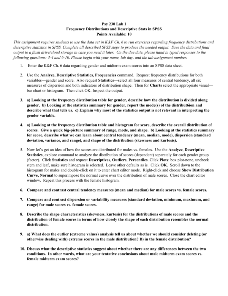
Psy 230 Lab 1
Frequency Distributions and Descriptive Stats in SPSS
Points Available: 10
This assignment requires students to use the data set in K&F Ch. 6 to run exercises regarding frequency distributions and
descriptive statistics in SPSS. Complete all described SPSS steps to produce the needed output. Save the data and final
output to a flash drive/cloud storage in case you need it later. On the due date, please hand in typed responses to the
following questions: 3-4 and 6-10. Please begin with your name, lab day, and the lab assignment number.
1.
Enter the K&F Ch. 6 data regarding gender and midterm exam scores into an SPSS data sheet.
2. Use the Analyze, Descriptive Statistics, Frequencies command. Request frequency distributions for both
variables—gender and score. Also request Statistics—select all four measures of central tendency, all six
measures of dispersion and both indicators of distribution shape. Then for Charts select the appropriate visual—
bar chart or histogram. Then click OK. Inspect the output.
3. a) Looking at the frequency distribution table for gender, describe how the distribution is divided along
gender. b) Looking at the statistics summary for gender, report the mode(s) of the distribut6ion and
describe what that tells us. c) Explain why most of the statistics output is not relevant in interpreting the
gender variable.
4. a) Looking at the frequency distribution table and histogram for score, describe the overall distribution of
scores. Give a quick big-picture summary of range, mode, and shape. b) Looking at the statistics summary
for score, describe what we can learn about central tendency (mean, median, mode), dispersion (standard
deviation, variance, and range), and shape of the distribution (skewness and kurtosis).
5. Now let’s get an idea of how the scores are distributed for males vs. females. Use the Analyze, Descriptive
Statistics, explore command to analyze the distribution of scores (dependent) separately for each gender group
(factor). Click Statistics and request Descriptives, Outliers, Percentiles. Click Plots: box plot-none, uncheck
stem and leaf, make sure histogram is selected. Leave other defaults as is. Click OK. Scroll down to the
histogram for males and double-click on it to enter chart editor mode. Right-click and choose Show Distribution
Curve, Normal to superimpose the normal curve over the distribution of male scores. Close the chart editor
window. Repeat this process with the female histogram.
6. Compare and contrast central tendency measures (mean and median) for male scores vs. female scores.
7. Compare and contrast dispersion or variability measures (standard deviation, minimum, maximum, and
range) for male scores vs. female scores.
8. Describe the shape characteristics (skewness, kurtosis) for the distributions of male scores and the
distribution of female scores in terms of how closely the shape of each distribution resembles the normal
distribution.
9. a) What does the outlier (extreme values) analysis tell us about whether we should consider deleting (or
otherwise dealing with) extreme scores in the male distribution? B) in the female distribution?
10. Discuss what the descriptive statistics suggest about whether there are any differences between the two
conditions. In other words, what are your tentative conclusions about male midterm exam scores vs.
female midterm exam scores?