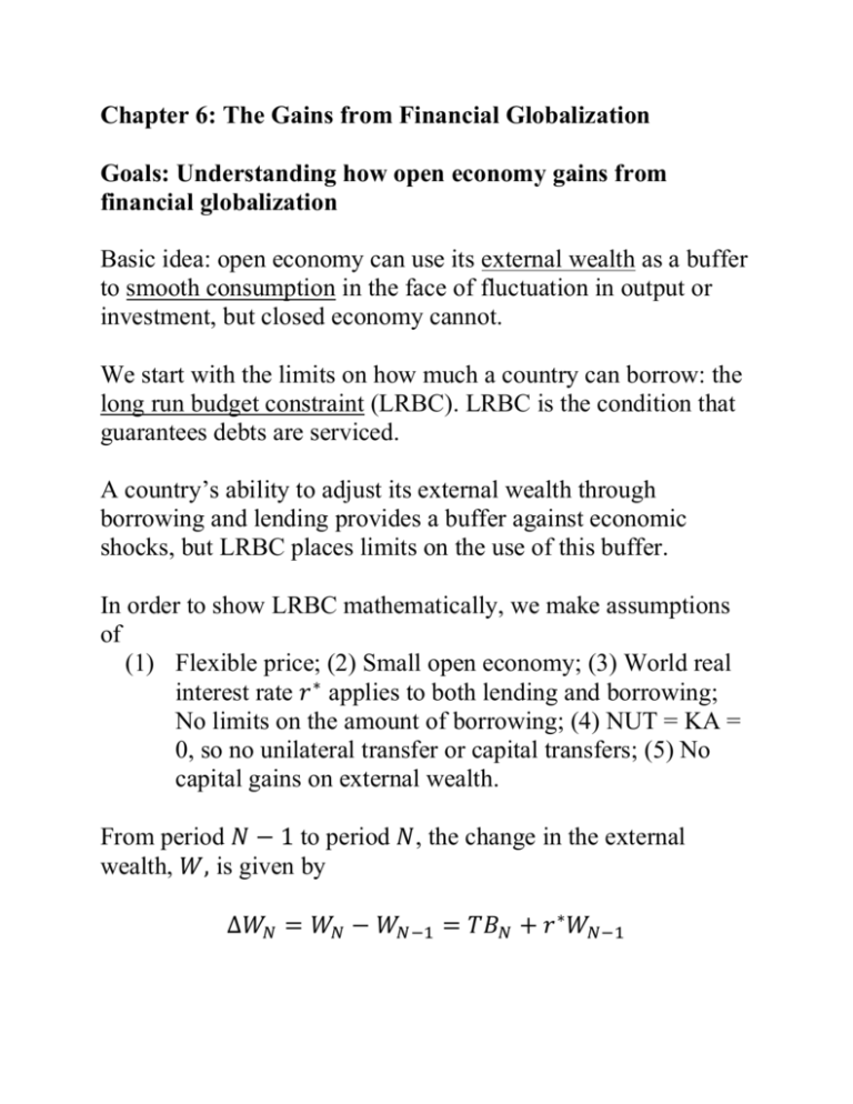
Chapter 6: The Gains from Financial Globalization
Goals: Understanding how open economy gains from
financial globalization
Basic idea: open economy can use its external wealth as a buffer
to smooth consumption in the face of fluctuation in output or
investment, but closed economy cannot.
We start with the limits on how much a country can borrow: the
long run budget constraint (LRBC). LRBC is the condition that
guarantees debts are serviced.
A country’s ability to adjust its external wealth through
borrowing and lending provides a buffer against economic
shocks, but LRBC places limits on the use of this buffer.
In order to show LRBC mathematically, we make assumptions
of
(1) Flexible price; (2) Small open economy; (3) World real
interest rate 𝑟 ∗ applies to both lending and borrowing;
No limits on the amount of borrowing; (4) NUT = KA =
0, so no unilateral transfer or capital transfers; (5) No
capital gains on external wealth.
From period 𝑁 − 1 to period 𝑁, the change in the external
wealth, 𝑊, is given by
∆𝑊𝑁 = 𝑊𝑁 − 𝑊𝑁−1 = 𝑇𝐵𝑁 + 𝑟 ∗ 𝑊𝑁−1
where 𝑇𝐵 denotes trade balance (net export); 𝑟 ∗ 𝑊𝑁−1 is the
interest paid or received on last period’s external wealth.
Everything else equal, positive trade balance causes external
wealth (rises or falls).
Rearranging the preceding equation leads to
𝑊𝑁 = 𝑇𝐵𝑁 + (1 + 𝑟 ∗ )𝑊𝑁−1
So external wealth at the end of this period equals trade balance
this period plus last period’s external wealth plus interest paid or
received.
We can get a sense of LRBC by looking first at a two-period
example. Suppose we start in year 0, so 𝑁 = 0. The initial
external wealth is 𝑊−1 . By the end of year 1, the country must
end all external borrowing or lending. That is, all debts owed or
owing must be paid off, and the country must end that year with
zero external wealth (𝑊1 = 0)
𝑊0 = 𝑇𝐵0 + (1 + 𝑟 ∗ )𝑊−1
0 = 𝑊1 = 𝑇𝐵1 + (1 + 𝑟 ∗ )𝑊0
These two equations jointly imply
0 = 𝑊1 = 𝑇𝐵1 + (1 + 𝑟 ∗ )𝑇𝐵0 + (1 + 𝑟 ∗ )2 𝑊−1
Or equivalently,
∗
−(1 + 𝑟 )𝑊−1
𝑇𝐵1
= 𝑇𝐵0 +
(1 + 𝑟 ∗ )
This is the present value form of two-period LRBC.
More generally, when 𝑁 goes to infinity, the present value form
of LRBC is
−(1 + 𝑟 ∗ )𝑊−1
𝑇𝐵1
𝑇𝐵2
= 𝑇𝐵0 +
+
+⋯
(1 + 𝑟 ∗ ) (1 + 𝑟 ∗ )2
− 1)
(6
On the left hand side of LRBC is minus the present value of
initial external wealth. On the right hand side is the present
value of all present and future trade balances. LRBC rules out
exploding positive or negative external wealth.
Exercise: if 𝑊−1 > 0, on average, 𝑇𝐵 ( > or
<)0
Exercise: Consider a two-period example with 𝑊−1 = 0. Show
that 𝑇𝐵0 and 𝑇𝐵1 must have opposite signs.
Recall that TB = GDP – GNE, so we can rewrite (6-1) as
𝐺𝐷𝑃1
𝐺𝐷𝑃2
(1 + 𝑟 )𝑊−1 + 𝐺𝐷𝑃0 +
+
+⋯
(1 + 𝑟 ∗ ) (1 + 𝑟 ∗ )2
𝐺𝑁𝐸1
𝐺𝑁𝐸2
= 𝐺𝑁𝐸0 +
+
+⋯
(1 + 𝑟 ∗ ) (1 + 𝑟 ∗ )2
∗
(6 − 3)
The left hand side of (6-3) is the present value of the country’s
total resources; the right hand side is the present value of the
country’s total spending.
So LRBC (6-3) says that in the long run, in present value terms,
a country’s expenditure must equal its production plus any
initial wealth.
In a closed economy, “living with your means” requires a
country’s spending equal its income each and every year. In an
open economy, however, spending and income must be balanced
in a present value sense, rather than year by year.
This conclusion implies that an open economy ought to be able
to do better (or no worse) than a closed economy in achieving its
desired pattern of expenditure over time. This is the essence of
theoretical argument that there are gains from financial
globalization.
For a big country such as US, the formula for the change of
external wealth should be modified as
∆𝑊𝑁 = 𝑊𝑁 − 𝑊𝑁−1 = 𝑇𝐵𝑁 + 𝑟 ∗ 𝐴𝑁−1 − 𝑟 0 𝐿𝑁−1 + 𝐾𝐺
= 𝑇𝐵𝑁 + 𝑟 ∗ 𝑊𝑁−1 + (𝑟 ∗ − 𝑟 0 )𝐿𝑁−1 + 𝐾𝐺
where 𝑟 ∗ 𝐴𝑁−1 is the (higher) interest received on external asset,
𝑟 0 𝐿𝑁−1 the (lower) interest paid on external liability, (𝑟 ∗ −
𝑟 0 )𝐿𝑁−1 the income due to interest differential (by borrowing
low and lending high), and 𝐾𝐺 is the capital gains (price
changes) on external wealth. The last equality follows because
𝑊 = 𝐴 − 𝐿 by definition.
When US try to avoid exploding negative external wealth, it can
use positive income from interest differential or positive KG to
offset a negative trade balance. See the application on page 207.
For developing countries, they must pay a rate higher than 𝑟 ∗ in
order to borrow money from ROW. Meanwhile, they can only
borrow limited amount of money. See the application on page
210.
The gains from consumption smoothing: the basic model
Assumptions: (1) GDP or output is denoted by Q, which is
produced each period using labor as the only input. Q is subject
to shocks. (2) There is a representative household. (3) GNE = C
(so no I or G). (4) 𝑊−1 = 0. (5) Small open economy that takes
𝑟 ∗ = 0.05 as given.
Exercise: for this special case, please show that LRBC (6-3)
becomes:
Present value of Q = Present value of C (6-4)
We compare a closed economy in which TB = 0 in all periods
and LRBC is automatically satisfied, to an open economy in
which TB does not have to be zero.
We must verify that LRBC is satisfied in an open economy.
Table 6-1, With no shocks
Exercise: show how to get the present value for GDP
Table 6-2: With temporary shocks, closed economy
Table 6-3: With temporary shocks, open economy
Excise: show how to get C = 99
Excise: show how to get TB0 = -20
Verify that the present value of trade balance equals zero (so
LRBC is satisfied)
Did you see a typo in Table 6-3?
The lesson is, when output fluctuates, a closed economy cannot
smooth consumption, but an open economy can.
More explicitly, in a closed economy, consumption must equal
output in each period. So output fluctuation immediately
generates consumption fluctuation. In an open economy, the
desired smooth consumption path can be achieved by running a
trade deficit (or borrowing money) during bad times and a trade
surplus during good times.
Discuss: how to apply what you learn so far to analyze the
economic situation in North Korea?
Discuss: what kind of empirical findings does not support the
gain from smooth consumption?
The gains from efficient investment: the basic model
Now the output is produced using both labor and capital. LRBC
becomes
Present value of Q = Present value of C + Present value of I
(6-5)
Exercise: derive (6-5) by yourself.
We assume that undertaking the investment would require an
expenditure of 16 units, and that in return the investment will
pay off in future years by increasing the country’s output by 5
units in year 1 and all subsequent years.
Table 6-4: Open economy with permanent shocks to output due
to new investment.
The present value of Q = ___________________________
The present value of I = ____________________________
The present value of C = ___________________________
In each year C = ___________________________
Comparing to Table 6-1 we see the country is better off because
C remains smooth, and ____ higher than it was without the
investment.
Exercises:
TB0 = __________; TB1 = __________;
NFIA0 = __________; NFIA1 = __________;
CA0 = __________; CA1 = __________;
W0 = __________; W1 = __________;
Exercise: please construct Table 6-4 for a closed economy.
The conclusion is that the open economy is better off making the
investment and smoothing consumption, two goals that the
closed economy cannot simultaneously achieve.
More generally, a new investment requires ∆𝐾 units of output in
year 0. This investment will generate additional ∆𝑄 units of
output in year 1 and all later years.
The change in present value of output due to the investment =
_________________
The change in the present value of new investment =
___________________
LRBC implies that the change in present value of consumption
= ___________
The new investment will be undertaken only if the change in
present value of consumption is (positive or negative).
Mathematically, the condition for undertaking a new investment
is
∆𝑄
≥ 𝑟∗
∆𝐾
or the marginal product of capital (MPK) is at least as great as
the marginal cost, the real interest rate.
Application: delinking saving from investment
In closed economy investment must be financed by saving (or a
decrease in consumption).
In open economy, investment can be financed by deficit in CA
(or borrowing from ROW), and consumption can be smooth
(unchanged), see Table 9-4. So investment and domestic saving
are delinked in open economy.
Gains from diversification of risks (optional)
Plot of volatility of capital income against the share of the
portfolio devoted to foreign capital
In real world, not all shocks are asymmetric. The impact of
common shocks cannot be lessened by diversification.