Group Project 6 – Investigation of Response Features
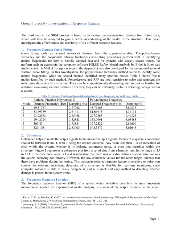
The third step in the SHM process is based on extracting damage-sensitive features from tested data,
which will then be analyzed to gain a better understanding of the health of the structure1. This paper
investigates the effectiveness and feasibility of six different response features.
1. Frequency Domain Curve Fitting
Curve fitting tools can be used to extract features from the experimental data. The polyreference
frequency and the polynomial rational fraction-z curve-fitting procedures perform well in identifying
natural frequencies for light to heavily damped data and for systems with closely spaced modes. To
perform such an extraction, the computer software PULSE Reflex Modal Analysis by Brüel & Kjær was
implemented. A MatLAB script (as seen in the Appendix) was also developed for the polynomial rational
fraction curve fitting. In this investigation, the polyreference frequency method failed to identify some
natural frequencies, while the second method identified many spurious modes. Table 1 shows first 6
modes identified by each method. Polyreference and RFP are both sensitive to noise and represent the
underlying dynamics of a structure. They can be computationally demanding and are not as feasible for
real-time monitoring as other features. However, they can be extremely useful in detecting damage within
a system.
Table 1. Rational fraction polynomial and polyreference frequency curve-fitting results
Rational Fraction Polynomial-Z
Mode Damped Frequency (Hz) Damping (%)
1
49.31767
3.77062
2
83.69389
2.61411
3
93.92983
2.65468
4
294.2724
3.32843
5
307.47
3.73831
6
329.1031
2.83005
Polyreference Frequency
Damped Frequency (Hz)
48.76165
81.66915
297.7363
333.0991
377.2522
543.3877
Damping (%)
3.80878
1.34111
4.44323
3.03485
2.84609
5.61648
2. Coherence
Coherence helps to relate the output signals to the measured input signals. Values of a system’s coherence
should be between 0 and 1, with 1 being the desired outcome. Any value less than 1 is an indication of
error within the system, whether it is leakage, extraneous noise, or even non-linearities within the
structure2. Figure 1 represents a coherence plot from a set of data from a hammer test. In the range of 25
to 65 Hz, the coherence value is 1 and is indicative that there was no extra instrumentation noise nor was
the system behaving non-linearly. However, the low coherence values for the other ranges indicate that
there were problems during the testing. This particular selected response feature is sensitive to noise, can
convey the relevant underlying dynamics of a structure, is feasible for real-time monitoring since
computer software is able to easily compute it, and is a quick and easy method to detecting whether
damage is present in the system or not.
3. Frequency Response Function
The frequency response function (FRF) of a system, which Avitabile considers the most important
measurement needed for experimental modal analysis, is a ratio of the output response to the input
1
Farrar, C. R., & Worden, K. (2007). An introduction to structural health monitoring. Philosophical Transactions of the Royal
Society A: Mathematical, Physical and Engineering Sciences, 365(1851), 303-315.
2
Allemang, R. J. (2001). Vibrations: Experimental Modal Analysis; Structural Dynamics Research Laboratory; University of
Cincinnati. UC-SDRL-CN-20-263-663/664.
Page | 1
response. Here, to quantitatively represent the characteristics of the FRF, the area under the curve of FRF
will be employed, computed as: Area FRF( f )df . The effectiveness of this FRF measure can be
easily illustrated using the following example, shown in Figure 2. Although there is no distinct variation
of the resulting FRF between two tests, a considerable variation of that computed Area is noticed: the
area under FRF of Test 2 is less than that of Test 1, and that difference, which can be approximated to
2.1%, can’t be neglected. The frequency response function is sensitive to noise and can reflect the
underlying dynamics of a structure. The FRF is an efficient procedure and is able to be used during
real time monitoring. Overall, the FRF is an important feature for experimental modal analysis and
is helpful for detecting damage within a system.
Figure 1: Coherence of hammer testing
90
80
Magnitude
70
60
50
40
30
20
10
0
0
50
100
Frequency (Hz)
150
200
Figure 2: Illustrative example to demonstrate the effectiveness using the area under the curve of FRF to feature the FRF
4. Modal Assurance Criterion (MAC)
MACis an experimental modal analysis tool used to help identify damage within a system. MAC, which
is a statistical indicator, is a leased squares based form of linear regression analysis3. The computer
software PULSE Reflex Modal Analysis by Brüel & Kjær was used to perform this analysis. Figure 3
represents the MAC information that was obtained. MAC is not very sensitive to noise and can reflect the
underlying dynamics of a structure. Although MAC requires numerous computational requirements and is
not feasible for real time monitoring, it can be a very helpful tool in detecting damage within a system,
especially when comparing a numerical model of a plate to measured data.
3
Pastor, M., Binda, M., & Harčarik, T. (2012). Modal assurance criterion. Procedia Engineering, 48, 543-548.
Page | 2
543.4
0.00
0.01
0.00
0.01
0.03
1.00
Polyreference Frequency
Modes
48.8
81.7
297.7
333.1
377.3
543.4
Polyreference Frequency
48.8 81.7 297.7 333.1 377.3
1.00 0.00 0.01 0.00 0.01
0.00 1.00 0.01 0.02 0.01
0.01 0.01 1.00 0.05 0.01
0.00 0.02 0.05 1.00 0.03
0.01 0.01 0.01 0.03 1.00
0.00 0.01 0.00 0.01 0.03
Rational Fraction Polynomial-Z
Modes 49.5 62.5 87.8 94.7 291.3 295.5
48.8 1.00 0.29 0.01 0.05 0.02 0.01
81.7 0.00 0.54 0.99 0.87 0.59 0.28
297.7 0.01 0.01 0.00 0.02 0.14 0.21
333.1 0.00 0.18 0.02 0.10 0.18 0.43
377.3 0.01 0.12 0.01 0.08 0.01 0.06
543.4 0.00 0.02 0.01 0.02 0.08 0.08
Figure 3: MAC for Polyref curve fitting (left) and CrossMAC for comparing RFP and Polyref (right)
5. Log decrement
Estimating the dampening coefficient of the time history data can be done using the log decrement
method across the duration of the response. The extracted dampened value is that of an analogous single
degree of freedom system. Figure 4 presents a log decrement procedure that has been performed. Log
decrement is not sensitive to noise and cannot reflect the underlying dynamics of a structure. It does
require computational requirements and is therefore not typically used during real time monitoring. Log
decrement is an efficient tool in detecting damage within a structure.
Figure 4: Log decrement results
6. Temporal moments
Temporal moments, analogous to statistical moments, are numerical values that are descriptive of the
overall nature of the output waveform. Each order represents a different temporal moment, with k = 0 – 4
being most common for Structural Health Monitoring applications. The temporal moments for these
orders are, Energy, Central Time, RMS Duration, Skewness, and Kurtosis, respectively. The following
table (Table 2) shows the temporal moments for the fifth test, accelerometers one and five. Temporal
moments are not sensitive to noise and can reflect the underlying dynamics of the structure. There are
some computational requirements making them not ideal for real-time monitoring. However, temporal
moments can be extremely useful in detecting damage within a system.
Table 2: Temporal Moments for the Fifth Test
Temporal Moment
Energy
Central Time
RMS Duration
Skewness
Kurtosis
Accelerometer 1
0.0274
0.3741
7.2783
162.43
3.89E+03
Accelerometer 5
0.0336
0.5244
10.8442
252.7172
6.16E+03
Page | 3
Appendix
MatLAB Rational Fraction Polynomial curve fitting for the frequency domain data
function mainrfp
rec=xlsread('Datatest.xls'); %get the test data, which contains the mangitude
%of each node for each frequency domain
omega=xlsread('Omega.xls'); %get the frequency domain
[alpha,par]=rfp(rec(:,1),omega,15);%the number of 15 is selected that 15
%natural frequency will be generated; and this function is to fit the
%tested frequency spectrum
plot(omega,rec(:,1),'r'), hold on;% plot the figure of test data on node #1;
%here,the number of 1 is selected to figure the frequency response spectrum
%of node #1
xlabel('Frequency (rad/sec)'),ylabel('Magnitude (dB)'),%plot the x and y
%lable of the figure
plot(omega,20*log10(abs(alpha)),'b'), hold off,%plot the estiamted frequency
%response spectrum of node #1
xlswrite('Node1.xlsx',par);%write the estimated natural frequency, damping
%ration, and etc. in to a xlsx file
end
Shown in below is an illustrative application of the MatLab code in the Appendix:
140
80
Test data
Fitted curve
60
Test data
120
Fitted curve
100
40
Magnitude (dB)
Magnitude (dB)
80
20
0
60
40
20
-20
0
-40
-20
-40
-60
-80
0
-60
1000
200
400
600
Frequency (rad/sec)
800
1000
3 modes (frequency from 0 to 1000 Hz)
1200
1400
1600
1800 2000 2200 2400
Frequency (rad/sec)
2600
2800
3000
3200
8 modes (frequency from 1000 to 3200 Hz)
Page | 4