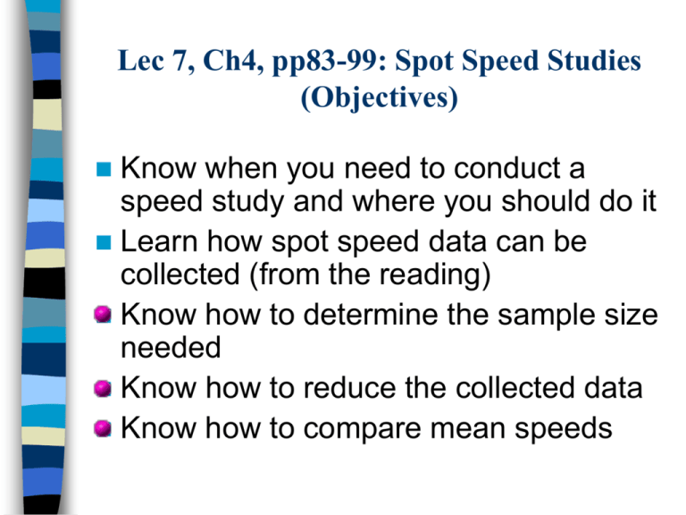
Lec 7, Ch4, pp83-99: Spot Speed Studies
(Objectives)
Know when you need to conduct a
speed study and where you should do it
 Learn how spot speed data can be
collected (from the reading)
 Know how to determine the sample size
needed
 Know how to reduce the collected data
 Know how to compare mean speeds

What we cover in class today…
Use of spot speed studies and time and
locations to choose
 Methods for conducting spot speed
studies
 The formula to determine the sample
size
 How to compute descriptive statistics
 How to compare two mean speeds

When are spot speed studies needed?
Spot speed studies are conducted to estimate the
distribution of speeds of vehicles in a stream of traffic
at a particular location on a highway.
Speed
Limit
Used for:
50
 Establish speed zones
 Determine whether complaints about speeding are valid
 Establish passing and no-passing zones
 Design geometric alignment
 Analyze accident data
 Evaluate the effects of physical improvements, etc., etc.
Location, time of day, and duration…
The objective and scope of the study
dictate these.
Basic data collection
Like deciding speed limits  Find
locations where system
characteristics change and TWTh
Speed trend analyses Avoid external influences such as
traffic lights, busy access roads; offpeak, TWTh  mid blocks of streets,
straight,level sections of highways
Specific traffic
All other specific purposes 
engineering problems Conduct it at the location of interest
and time of day
At least 1 hour and at least 30 data (if you want to assume
normal distribution)
Descriptive statistics of speed data
Once data are collected, the first thing you do is to compute
several descriptive statistics to get some ideas about the
distribution of the speed data. (Note that many statistical analyses
used in traffic engineering assume data are normally distributed.
 So, the goal is to check whether they are really normally
distributed.
Typical descriptive statistics are:
 Average speed
 Variance and standard deviation
 Median speed
 Modal speed (or Modal speed range  Needs a histogram)
 The ith-percentile spot speed
 Pace  Usually a 10-mph interval that has the greatest
number of observations.
Descriptive statistics (cont.)
Average
speed
Speed data
Grouped
Not grouped
u = uj/N
Standard
deviation
Speed data
Grouped
s=
f(ui – u)2
N-1
Variance
s2
Not grouped
Descriptive statistics (cont)
Median speed The speed at the middle value in a series of spot
speeds. Or, 50th-percentile speed
Modal speed
The speed value that occurs most frequently in a
sample of speeds
ith-percentile
speed
The spot speed below which i percent of the
vehicles travel, e.g. 85th-percentile speed
Pace
The range of speed that has the greatest number
of observations; usually 10-mph range
85%
50%
Determining the sample size… (p.89)
Need to know a bit of statistical principles here…
It’s all based on the normal distribution curve.
d
N = Min. sample size
Z α/2 = 1.96 for 95% conf. Level
68.3%
2
Frequency
N=
Zα/2 
95.0%
 = Estimated standard deviation
Rural 2-lane: 5.3 mph
Rural 4-lane: 4.2 mph
-/sqrt(n)  +/sqrt(n)
-1.96/sqrt(n)
+1.96/sqrt(n)
Urban 2-lane: 4.8 mph
Urban 4-lane: 4.9 mph
d = Precision level (depends on the study)
At 95% Confidence level, Z =
1.96 (This is the most important
number to remember.)
Example 4.2 by spreadsheet (Click Example
4.2 in the lecture schedule.)
Comparing two mean speeds
This test is done to compare the effectiveness of an
improvement to a highway or street by using mean speeds.
 If you want to prove that the difference exists
between the two data samples, you conduct a twoway test. We discuss only this one in this class.
Null hypothesis H0: 1 = 2
Alternative H1: 1 = 2
 If you are sure that the improvement would
improve the performance of the highway or street,
you conduct a one-way test. This will be discussed
in CE562.
Alternative H1: 1  2
Comparing two mean speeds (cont)
Step 1: Find mean and SD of the two samples
u1 = 35.5 mph
S1 = 7.5 mph
n1 = 250
u2 = 38.7 mph
S2 = 7.4 mph
n2 = 280
Step 2: Compute the standard deviation of the difference in
means (Assumes S12 and S22 are similar)
Sd = SQRT(S12/n1 + S22/n2) = SQRT(7.52/250 + 7.42/280) = 0.65
Step 3: Test the hypothesis. If |u1- u2| > ZSd, the mean speeds
are significantly different at the confidence level of Z.
|35.5 – 38.7| = 3.2 mph > 1.96*0.65 = 1.3mph
It can be concluded that the difference in mean speeds is
significant at the 95% confidence level.