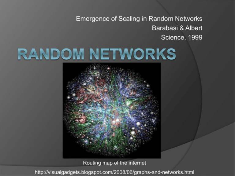
Emergence of Scaling in Random Networks
Barabasi & Albert
Science, 1999
Routing map of the internet
http://visualgadgets.blogspot.com/2008/06/graphs-and-networks.html
What is a network?

A graph is : an ordered pair G = (V,E)
comprising a set V of vertices or nodes
together with a set E of edges or lines,
which are 2-element subsets of V

A set of elements together with
interactions between them

Representation: a set of dots connected
with (directed) lines
Where networks arise?

Computer networks
 Internet, LAN, Token-ring, 1553

Biology
 Gene regulation, food chain, metabolic networks

Data storage structures:
 WWW, data-base trees

Power transmition
 Electric power grid, hydraulic transmition

Social interaction
 Citation patterns, friendships, professional hierarchy

Computation
 Flow field computation, stress field computation
Internet routing map, 1999
http://www.cheswick.com/ches/map/
Power grid, USA, 2001
http://www.technologyreview.com/Energy/12474/page2/
Sexual / Romantic partners
network
Bearman, Moody, Stovel. Chains of Affection: The Structure of Adolescent
Romantic and Sexual Networks. AJS, 2004
Jefferson High, Columbus, Ohio
Metabolic network of E. Coli
Organization chart
Large-scale, “natural” networks

How “random” are “natural” networks
(WWW, internet, gene regulation, …)
 “natural” ~ no apriori structure defined

What are the key characteristics of natural
networks?
What is “Random Network”?

Random network – ensemble of many
possible networks:
 Fixed or unfixed number of vertices (dots)
 Fixed or unfixed number of edges (lines)
 Any two vertices have some probability of being
connected

Key notion: node connectivity
 connectivity = number of connections

First model – Erdos & Renyi, 1947
ER random network model

Network model: a random network between n
nodes:
 Fix the number of vertices to n
 For each possible connection between vertices v
and u, connect with probability p

P(rank=k) =
ER random network model

Features
 Every node has appr.
same number of
connections
 connectivity is scaledependent!
l=l(N)
 Tree-like!
Internet-like network evolution
http://www.cheswick.com/ches/map/index.html
http://www.cheswick.com/ches/map/movie.mpeg
ER model and real life

Real-life networks are scale-free:
 Connectivity follows power-law: P(k) ~ kγ
γ = 2.1…4
○ very low connection numbers are possible
Actor collaboration
WWW
Power grid
N=212e3, <k>=29, γ=2.3
N=325e3, <k>=5.5, γ=2.1
N=5e3, <k>=2.7, γ=4
ER model VS. Scale-free
network


ER: same average number of connections per node – treelike
SF: hubs present – few nodes with large number of
connections – hierarchy!
ER model VS. Scale-free
network

Adjacency matrix A:
 Number the nodes from 1 to N
 If vp connected to vq , put 1 in apq
1
2
3
4
5
6
1
2 3
4
5
6
ER model VS. Scale-free
network
Adjacency matrix of ER: ~ uniform
distribution of 1’s
 Adjacency matrix of SF: 1’s lumped in
columns & rows for few nodes
SF
ER

Barabasi model

Goal: generation of random network
with “scale-free” property
1.
Number of edges – not fixed
 Continuous growth
2.
Preferential attachment
 Prob. of a new node to attach to existing one
rises with rank of node
P(attach to node V) ~ rank(V)
Barabasi Model
 Produces
scale-free networks
 Scale-free distribution – time-invariant.
Stays the same as more nodes added
Barabasi Model

Removal of either assumptions destroys
scale-free property:
 Without node addition with time → fully
connected network after enough time
 Without preferential attachment →
exponential connectivity
ER Vs. Barabasi

Graph diameter:
 the average length of shortest distance
between any two vertices

For same number of connections and
nodes, ER has larger diameter than
scale-free networks
 No small-world in ER!
Scale-free Network features
Network diameter
Failure =
removal of
random node
Attack =
removal of
highlyconnected node
% of “damaged” nodes
Robustness to random failure
 Susceptibility to deliberate attack

Scale-free Network features

“Small-world” phenomenon, or:
“6 degrees of separation”

Stanley Milgram, 1967, Psychology today
Small-world experiment

Experiment: send a package from
Nebraska and Kansas (central US) to
Boston, to a person the sender doesn’t
know
 Motivation: great distance – social and
geographical

Only 64 of 296 packages were delivered

For delivered packages: average path
length ~ 6
Google search
Brin & Page, 1998; Kleinberg, 1999

Pages are ranked according to incoming
links
 Incoming link from a high-score page is more
valuable

Meaning: after random clicks, a user will be
on high-ranked page

Prefers old, well-connected pages
Google search
Erdos & Bacon Number

Erdos number: “collaborative distance”
of a mathematician from Paul Erdos
 Average: ~6
 Kahenman, Auman: 3

Bacon Number: “collaborative distance”
of an actor from Kevin Bacon
 http://oracleofbacon.org/
 Average: ~3
Summary

Many real-life, large-scale networks exhibit a
scale-free distribution of connectivity

Distribution is power-law
 Similar powers for networks of different types
 Small-world phenomenon

Key features to enable free-scale property:
 Addition of new nodes
 Preferential attachment