Business and
Economic Forecasting
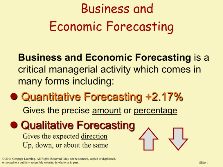
Business and Economic Forecasting is a
critical managerial activity which comes in
many forms including:
Quantitative Forecasting +2.17%
Gives the precise amount or percentage
Qualitative Forecasting
Gives the expected direction
Up, down, or about the same
© 2011 Cengage Learning. All Rights Reserved. May not be scanned, copied or duplicated,
or posted to a publicly accessible website, in whole or in part.
Slide 1
The Significance of Forecasting
• Both public and private enterprises operate under
conditions of uncertainty.
• Management wishes to limit this uncertainty by
predicting changes in cost, price, sales, and interest
rates.
• Accurate forecasting can help develop strategies to
promote profitable trends and to avoid unprofitable
ones.
• A forecast is a prediction concerning the future. Good
forecasting will reduce, but not eliminate, the
uncertainty that all managers feel.
Slide 2
Hierarchy of Forecasts
• The selection of forecasting techniques depends in part on the level of
economic aggregation involved.
• The hierarchy of forecasting is:
• National Economy (GDP, interest rates, inflation, etc.)
» Sectors of the economy (durable goods)
Industry forecasts (all automobile manufacturers)
Firm forecasts (Ford Motor Company)
o Product forecasts (The Ford Focus)
Slide 3
Criteria Used to Select a Technique
1.
2.
3.
4.
5.
The choice of a particular forecasting method
depends on several criteria:
costs of the forecasting method compared with its
gains
complexity of the relationships among variables
time period involved
lead time between receiving information and the
decision to be made
accuracy of the forecast
Slide 4
Accuracy of Forecasting
• The accuracy of a forecasting model is measured by how
close the actual
variable, Y, ends up to the forecasting
variable, Y .
• Forecast error is the difference. (Y -Y)
• Models differ in accuracy, which is often based on the
square root of the average squared forecast error over a
series of N forecasts and actual figures
• Called a root mean square error, RMSE:
1
2
RMSE
(
Y
Y
)
t
t
n
Slide 5
ALTERNATIVE FORECASTING
TECHNIQUES
• Alternative forecasting techniques can be classified in the
following general categories:
»
»
»
»
»
»
»
Deterministic trend analysis
Smoothing techniques
Barometric indicators
Survey and opinion-polling techniques
Macroeconometric models
Stochastic time-series analysis
Forecasting with input-output tables
Slide 6
Deterministic Trend Analysis
• Time-series data. A series of observations taken
on an economic variable at various past points in
time.
»
»
»
»
Secular trends
Cyclical variations
Seasonal effects
Random fluctuations
• Cross-sectional data. Series of observations taken
on different observation units (for example,
households, states, or countries) at the same point
in time.
» Ratio to trend method
» Dummy variables
Slide 7
FIGURE 5.2 Secular, Cyclical, Seasonal, and
Random Fluctuations in Time Series Data
Slide 8
FIGURE 5.2 Secular, Cyclical, Seasonal, and
Random Fluctuations in Time Series Data
Slide 9
Elementary Time Series Models
for Economic Forecasting
^
Yt+1 = Yt
» The simplest method
» Best when there is no
trend, only random
error
» Graphs of sales over
time with and without
trends
» When trending down,
the simplest predicts
too high
NO Trend
time
Trend
time
Slide 10
Slide 11
Secular Trends
^ = Y + (Y - Y )
Y
t+1
t
t
t-1
» This equation begins with last period’s forecast, Yt, just
like the simple forecast.
» Plus an ‘adjustment’ for the change in the amount
between periods Yt and Yt-1.
» When the forecast is trending up or down, this
adjustment works better than the simple forecast
method #1.
Slide 12
Deterministic Trend Analysis
Components of Time Series
Dependent Variable
X
X
X
Forecasted Amounts
T0
TIME
The data may offer secular trends, cyclical variations, seasonal
variations, and random fluctuations.
Slide 13
Time Series
Examine Patterns in the Past
Dependent Variable
Secular Trend
X
X
X
Forecasted Amounts
T0
TIME
The data may offer secular trends, cyclical variations, seasonal
variations, and random fluctuations.
Slide 14
Time Series
Examine Patterns in the Past
Dependent Variable
Cyclical and Seasonal Variation
Secular Trend
X
X
X
Forecasted Amounts
T0
TIME
The data may offer secular trends, cyclical variations, seasonal
variations, and random fluctuations.
Slide 15
Linear Trend & Constant Rate of
Growth Trend
Linear Trend Growth
• Used when trend has a
constant AMOUNT of
change
Yt = a + b•T, where
Yt are the actual
observations and
T is a numerical time
variable
Uses a Semi-log Regression
• Used when trend is a
constant
PERCENTAGE rate
Log Yt = a + b•T,
where b is the
continuously
compounded growth
rate
Slide 16
FIGURE 5.4 Prizer Creamery: Monthly Ice Cream Sales
Slide 17
More on Constant Rate of Growth
Model – a proof
^
• Suppose: Yt = Y0( 1 + g) t where g is the
annual growth rate
• Take the natural log of both sides:
^
» Ln Yt = Ln Y0 + t • Ln (1 + g)
» but Ln ( 1 + g ) g, the continuously
compounded growth rate
» SO:
Ln Yt = Ln Y0 + t • g
Ln Yt = a + b • t
where b is the growth rate, g.
Slide 18
Numerical Examples:
MTB > Print c1-c3.
Sales Time Ln-sales
100.0
109.8
121.6
133.7
146.2
164.3
1
2
3
4
5
6
4.60517
4.69866
4.80074
4.89560
4.98498
5.10169
6 observations
Using this sales
data, estimate
sales in period 7
using a linear and
a semi-log
functional
form
Slide 19
The linear regression equation is
Sales = 85.0 + 12.7 Time
Predictor Coef
Constant
84.987
Time
12.6514
s = 2.596
Stdev
2.417
0.6207
R-sq = 99.0%
t-ratio p
35.16 0.000
20.38 0.000
R-sq(adj) = 98.8%
The semi-log regression equation is
Ln-sales = 4.50 + 0.0982 Time
Predictor Coef
Stdev
Constant 4.50416 0.00642
Time
0.098183 0.001649
s = 0.006899
R-sq = 99.9%
t-ratio
p
701.35 0.000
59.54 0.000
R-sq(adj) = 99.9%
Slide 20
Forecasted Sales @ Time = 7
• Linear Model
• Sales = 85.0 + 12.7 Time
• Sales = 85.0 + 12.7 ( 7)
• Sales = 173.9
• Semi-Log Model
• Ln-sales = 4.50 + 0.0982
Time
• Ln-sales = 4.50 +
0.0982 ( 7 )
• Ln-sales = 5.1874
• To anti-log:
linear
» e5.1874 = 179.0
Slide 21
Sales Time Ln-sales
Semi-log is
exponential
100.0
109.8
121.6
133.7
146.2
164.3
179.0
173.9
1
2
3
4
5
6
4.60517
4.69866
4.80074
4.89560
4.98498
5.10169
7 semi-log
7 linear
7
Which prediction
do you prefer?
Slide 22
Declining Rate of Growth Trend
• A number of marketing penetration models
use a slight modification of the constant rate
of growth model
• In this form, the inverse of time is used
Ln Yt = b1 – b2 ( 1/t )
• This form is good for patterns
like the one to the right
• It grows, but at continuously
a declining rate
Y
time
Slide 23
Seasonal Adjustments: The Ratio to Trend Method
12 quarters of data
1 2 3 41 2 3 41 2 3 4
Take ratios of the actual (A) to
the forecasted (F) values for
past years.
A1/F1, A2/F2, A3/F3, find
average of these ratios.
This is the seasonal adjustment
Adjust by this percentage by
multiply your forecast by the
seasonal adjustment
» If average ratio is 1.02,
adjust forecast upward 2%
Slide 24
Seasonal Adjustments: Dummy Variables
• Let D = 1, if 4th quarter and 0 otherwise
• Run a new regression:
Yt = a + b•T + c•D
» the “c” coefficient gives the amount of the adjustment for the
fourth quarter. It is an Intercept Shifter.
» With 4 quarters, there can be as many as three dummy variables;
with 12 months, there can be as many as 11 dummy variables
• EXAMPLE: Sales = 300 + 10•T + 18•D
12 Observations from the first quarter of 2008-I to 2010-IV.
Forecast all of 2011.
Sales(2011-I) = 430; Sales(2011-II) = 440; Sales(2011-III) = 450;
Sales(2011-IV) = 478
Slide 25
Smoothing Techniques: Moving Averages
• A smoothing forecast
method for data that
Dependent Variable
jumps around
• Best when there is no
*
*
trend
*
• 3-Period Moving Ave is:
*
^
Yt+1 = [Yt + Yt-1 + Yt-2]/3
• For more periods, add
them up and take the
average
*
Forecast
Line is
Smoother
TIME
Slide 26
FIGURE 5.6 Walker Corporation’s ThreeMonth Moving Average Sales Forecast Chart
Slide 27
Smoothing Techniques
First-Order Exponential Smoothing
• A hybrid of the Naive • Each forecast is a function of
and Moving Average
all past observations
methods
• Can show that forecast is
^
^ t+1 = w•Yt +(1-w)Yt
• Y
based on geometrically
declining weights.
• A weighted average of
^ = w •Y +(1-w)•w•Y +
past actual and past
Y
t+1
t
t-1
forecast, with a weight (1-w)2•w•Yt-2 + …
of w
Find lowest RMSE to pick the
best w.
Slide 28
First-Order Exponential
Smoothing Example for w = .50
1
2
3
4
5
Actual Sales
100
120
115
130
Forecast
100 initial seed required
.5(100) + .5(100) = 100
?
Slide 29
First-Order Exponential
Smoothing Example for w = .50
1
2
3
4
5
Actual Sales
100
120
115
130
Forecast
100 initial seed required
.5(100) + .5(100) = 100
.5(120) + .5(100) = 110
?
Slide 30
First-Order Exponential
Smoothing Example for w = .50
1
2
3
4
5
Actual Sales
100
120
115
130
?
Forecast
100 initial seed required
.5(100) + .5(100) = 100
.5(120) + .5(100) = 110
.5(115) + .5(110) = 112.50
.5(130) + .5(112.50) = 121.25
MSE = {(120-100)2 + (110-115)2 + (130-112.5)2}/3 = 243.75
RMSE = 243.75 = 15.61
Period 5
Forecast
Slide 31
Barometric Techniques
Slide 32
Barometric Techniques
Slide 33
Barometric Techniques
Direction of sales can be indicated by other variables.
PEAK
Motor Control Sales
peak
Index of Capital Goods
TIME
4 Months
Example: Index of Capital Goods is a “leading indicator”
There are also lagging indicators and coincident indicators
Slide 34
Average time given in months from reference peaks
Table 5.7
LEADING INDICATORS*
»
»
»
»
COINCIDENT
INDICATORS
M2 money supply (-14.2)
S&P 500 stock prices (-11.1)
» Nonagricultural payrolls
Building permits (-15.4)
(+.8)
Initial unemployment claims
» Index of industrial
(-12.9)
production (-1.1)
Contracts and orders for
» Personal income less
plant and equipment (-7.3)
transfer payment (-.4)
LAGGING INDICATORS
»
*http://www.nber.org
» Inventory to sales ratio (9.2)
» Prime rate (+2.0)
» Change in labor cost per unit
of output (+6.4)
Slide 35
Surveys and Opinion Polling Techniques
• New product ideas have no historical data, but surveys can
assess interest ( Would you buy a phone that is also a Swiss knife? )
• Macroeconomic surveys include:
» Plant and equipment expenditure plans (McGraw-Hill, National
Industrial Conference Board, US Department of Commerce, Fortune).
» Plans for inventory changes and sales expectations (US Department
of Commerce, McGraw-Hill, Dun and Bradstreet, and the National
Association of Purchasing Agents)
» Consumer expenditure plans (U of Michigan’s Survey Research
Center on plans to buy autos, called consumer sentiment)
• Sales Forecasting include:
» Sales force polling (sales people know what their customers are
saying)
» Surveys of consumer intentions (asking prior customer’s their
intentions for replacing appliances, windows, etc.)
Slide 36
Econometric Models
Single Equation Models
• Specify the variables in the model. One example is
attendance at NFL games involving 14 variables from
price, weather, domes, non-Sunday games, and winning
record at home.
• Estimate the parameters of a typical demand function:
» Qd = a + b•P + c•I + d•Ps + e•Pc
• But forecasts require estimates for future prices, future
income, etc.
• Often combine econometric models with time series estimates of the
independent variable.
Slide 37
Example:
Suppose demand estimate to be:
• Qd = 400 - .5•P + 2•Y + .2•Ps
» anticipate pricing the good at P = $20
» Income (Y) is growing over time, the estimate is: Ln
Yt = 2.4 + .03•T, and next period is T = 17.
• Y = e2.910 = 18.357
» The prices of substitutes are likely to be P = $18.
• Find Qd by substituting in predictions for P, Y, and Ps
• Hence Qd = 430.31
Slide 38
Econometric Models
Multi-Equation Models
• In market (and life) interrelationships may be complex.
• Macroeconomic models of national income often involve
several equations for consumption, GDP, investment and
government.
i. C = a1 + b1 (GDP – T) + e1
ii. I = a2 + b2Pt-1 + e2
iii. T = b3GDP + e3
iv. GDP = C + I + G
• Such models offer forecasts, but can be supplemented
with judgment of the forecasters.
Slide 39
Slide 40
Slide 41
Stochastic Time Series
• A little more advanced methods incorporate into time
series the fact that economic data tends to drift
yt = a + byt-1 + et
• In this series, if a is zero and b is 1, this is essentially
the naïve model. When a is zero, the pattern is called a
random walk.
• When a is positive, the data drift. The Durbin-Watson
statistic will generally show the presence of
autocorrelation, or AR(1), integrated of order one.
• One solution to variables that drift, is to use first
differences.
Slide 42
Random Walks Illustrated
Slide 43
Cointegrated Time Series
• Some econometric work includes several stochastic
variable, each which exhibits random walk with drift
» Suppose price data (P) has positive drift (trends up)
» Suppose GDP data (Y) has positive drift (trends up too)
» Suppose the sales is a function of P & Y
» Salest = a + bPt + cYt
» It is likely that P and Y are cointegrated in that they
exhibit co-movement with one another. They are not
independent.
» The simplest solution is to change the form into first
differences as in: DSalest = a + bDPt + cDYt
Slide 44
Managing in the
Global Economy
•
•
•
•
•
•
•
•
Import-Export Sales and Exchange Rates
The Market for US Dollars as Foreign Exchange
Foreign Exchange (FX) Risk Management
Determinants of the Long-Run Trends in Exchange Rates
Purchasing Power Parity
International Trade and Trading Blocs (EU & NAFTA)
Comparative Advantage and Trade
Trade Deficits and the Balance of Payments
© 2011 Cengage Learning. All Rights Reserved. May not be scanned, copied or duplicated,
or posted to a publicly accessible website, in whole or in part.
Slide 45
The Financial Crisis
and Exports to China
• The financial crisis in housing and banking led to a prolonged
recession
• US is largest at $14+ trillion; Japan at $5 trillion; China at $4.4
trillion; Germany at $3.7 trillion; and France at $2.8 trillion.
• Though a relatively small portion of US GDP (of 10% exports &
13% imports), exports and imports have been a driver of growth.
• Although both consumers and businesses cut back in
expenditures, exports to China continued.
• Solutions to global downturn involves expansionary fiscal and
expansionary monetary policies, although neither has been
especially successful thus far.
Slide 46
The Financial Crisis
and Exports to China
Slide 47
Import-Export Sales and Exchange Rates
• More and more firm are becoming
multinational enterprises.
• Exports and imports are influenced by
changes in international exchange rates.
• Differences in long run inflation rates
(according to the theory of purchasing power
parity), national economic growth rates, and
interest rates help explain long-term
exchange rate movements.
Slide 48
FIGURE 6.1 Foreign Exchange (FX) Rates: The Value of
the U.S. Dollar against Several Major Currencies
Slide 49
Competitiveness and Exchange Rates
• The international competitiveness of
products is affected by exchange rates.
• If the US exports a Jeep that sells for $30,000, the price of the same
car in Europe is vastly different
» In 2000, $/€ = $.86/€. If a US car costs $30,000, then in Euros
that is $30,000 / $.860/€ or €34,884.
When $/€ = $.86/€, then €/$ = 1/ $.86/€ = €1.163/$
» In 2010, $/€ = $1.32/€. If that same car costs $30,000, then in
Euros that is $30,000 / $1.32/€ or €22,727.
When $/€ = $1.32/€, then €/$ = 1/ $1.32/€ = €.757/$
» Clearly, more Jeeps are likely to be sold in Europe at the lower
than the higher price.
Slide 50
Foreign Exchange Risk Exposure
• Transaction Risk Exposure – occurs when a change in cash flows
results from contractual commitments to pay or receive a foreign
currency.
» When GE sells equipment to Japan in Yen, but they give 60 days before the
payment is due, there is a risk that the Yen will fall in value.
• Translation Risk Exposure – occurs when the value of foreign
assets or liabilities are affected by exchange rates.
» Disney owns a park near Paris. When the Euro rises against the dollar, the
value of the land rises in terms of dollars. This is primarily an accounting
adjustment.
• Operating Risk Exposure – occurs when cash flows of the firm are
impacted by exchange rates.
» When Jeep sells more Grand Cherokees when the value of the dollar is low,
and less when it is high, this is operating risk exposure. This is the most
important risk.
Slide 51
The Market for US Dollars as
Foreign Exchange
• Jeep, BMW, and Cummins Engine are buying
and selling foreign exchange in the market.
• Governments can also intervene through
buying or selling currencies that they hold.
• Spot Price for foreign exchange is current
price(2 day delivery) can appear in different
terms: $/€ or €/$, which is just the inverse.
Both are given in the Cross Rates.
• Forward Price is the price of a foreign
currency for delivery at a future date agreed by
contract today
Slide 52
FIGURE 6.2 Cummins Engine Cash
Flow and Operating Margins
Slide 53
Canadian Dollar
Spot and Forward Rates
August 6, 2010
http://fx.sauder.ubc.ca/CAD/forward.html
Country
Canada (C$) spot
1-month forward
3-months forward
6-months forward
US$ per 1C$
0.9730
0.9727
0.9715
0.9694
What does the market think will happen to the C$
based on the forward rates over the long run?
Slide 54
CROSS RATES 8-6-10
USD $
JPY ¥
EUR €
CAD $
GBP £
AUD $
CHF
1 USD $
–
85.435
0.7526
1.0273
0.6264
1.0891
1.0386
1 JPY ¥
0.0117
–
0.0088
0.012
0.0073
0.0127
0.0122
1 EUR €
1.3287 113.5198
–
1.365
0.8323
1.4471
1.38
1 CAD $
0.9734
0.7326
–
0.6098
1.0602
1.011
1 GBP £
1.5964 136.3905 1.2015
1.64
–
1.7387
1.658
1 AUD $
0.9182
78.4455
0.691
0.9433
0.5752
–
0.9536
1 CHF
0.9628
82.2598
0.7246
0.9891
0.6031
1.0486
–
83.1646
http://finance.yahoo.com/currency-investing#cross-rates
USD $ is the US dollar; JPY ¥ is the Japanese yen; EUR € is the European Euro; GBP is the
Slide 55
British pound; AUD $ is the Australian dollar; and CHF is the Swiss franc
Outsourcing
• Global firms seek lowest cost ways to produce
• When firms do one or more steps of their production
outside of their home country, we say that activity was
“outsourced”
• This can help firms survive that face stiff competition
from abroad by holding down their costs. In this
way, some jobs are saved while others leave this
country.
• Outsourcing is criticized as ‘exporting jobs.’
Slide 56
FIGURE 6.3 Outsourcing Shipping Costs and Component
Sources for HP Personal Computer
Slide 57
China Trade Blossoms
• Worldwide trade with China jumped from 4.2%
in 2003 to 8% in 2008, and is growing.
• China as joint ventures with global firms (Ford,
McDonnell-Douglas, HP, and many others).
• GDP in China grows at phenomenal rates
doubling in 5-7 years, and population growing at
1%, improving their standard of living.
• Liberalization of property rights and the creation
of a middle class are hallmark’s of moving from
a developing to a developed country.
Slide 58
The Market for Dollars
as Foreign Exchange
• Foreign Exchange is used
for trade and investment.
Use a supply & demand
model to explore FX
rates
• Demand for Swiss Francs
(SFr): Demand is associated
with US demand for imports
from Switzerland and
purchase of Swiss financial
securities
$/SFr
1,000 SFr
D
SFr
Slide 59
Supply of SFr
• Supply of SFr -Supply is associated
with SWISS demand
for US exports and US
financial investments.
• Market Clears-$/SFr
no excess demand or
excess supply of SF
• In Flexible Markets, buying
& selling through
international banks
S
$.9628
D
SFr
Slide 60
Suppose there is a rise in
US Inflation Rates
S'
• Both Supply & Demand of
SFr Shift
S
• SWISS products appear
cheaper, so D shifts to D′ $2/SFr
• US exports appear
more expensive, so
shifts from S to S′
$1/SFr
D'
• The SFr appreciates, and
the dollar depreciates
D
SFr
Slide 61
Suppose U.S. interest rates rise
• Supply of Swiss francs rises
as Swiss seek to invest in
the US from S to S′
• Demand for Swiss
investments declines, from
$1/SFr
D to D′
• Swiss francs fall in value and
the dollar rises in value
$2/SFr
• What happens when
Greenspan CUTS interest
rates?
S
S′
D
D'
Slide 62
Suppose US Economic Growth rises
• Supply of Swiss francs rises
as Swiss seek to invest in
the US from S to S′
• Demand for Swiss products
and services rise from D to
$1/SFr
D′ as growth increases
$2/SFr
appetite for everything.
• Swiss francs fall in value and
the dollar rises in value
• What happens when Swiss
growth rates rise?
S
S′
D'
D
Slide 63
FIGURE 6.4 The Market for U.S. Dollars as
Foreign Exchange (Depreciation of the Dollar,
2001–2008)
Slide 64
Governmental Intervention in Foreign
Exchange Markets
• Governments can and do intervene in markets
» Directly by buying and selling foreign currencies
» And indirectly by altering interest rates or inflation rates
• Sterilized Interventions involve offsetting an
indirect move (like an increase in short term
interest rates) through direct action in the
foreign currency markets
• Coordinated Interventions involve several
countries all agreeing to intervene to raise or
lower the exchange rate of some country.
Slide 65
Determinants of Long-Run Trends
in Exchange Rates
1. Countries that have high growth rates in
GDP tend to have rising currency values.
2. Countries that have relatively high real
(inflation-adjusted) interest rates, tend to
have rising currency values .
3. Countries with relatively high inflation
expectations tend to declining currency
values.
Slide 66
Slide 67
FIGURE 6.5 The Market for U.S. Dollars as
Foreign Exchange (Depreciation against the Yen,
2007–2009, and the Euro, 2001–2008)
Slide 68
Purchasing Power Parity (PPP)
• Purchasing power parity says that the price of
traded goods tends to be equal around the world.
This is: the law of one price.
» if exchange rates are flexible and there are no
significant costs or barriers to trade, then:
Relative PPP [6.1]:
S1 = ( 1 + h )
S0 ( 1 + f )
S1/S0 shows the expected change in the direct quote of a
currency. The right side of the equation is the ratio of home and
foreign inflation rates. If the foreign inflation rises (f), then the
domestic expected future spot rates S1 declines.
Slide 69
Slide 70
PPP Example
• Suppose inflation in the US is 3%
• Suppose that inflation in Canada is 4%
• The currency price of the Canadian dollar is
$.973/C$.
• What is the expected price of the Canadian dollar
in one year?
• Answer:
S1 = ( 1 + h ) = 1.03 = .9903 = S1
S0 ( 1 + f ) 1.04
.973
• Hence, S1 = .973*.9903 = $ 0.9636/C$, a slight
decline from $.973.
Slide 71
PPP As Yardstick Of Comparative Growth
• PPP can be used to compare growth rates
• An “implied FX” rate is the ratio of prices of like items
in two countries, say iPods sold in US and UK.
» A $225 iPod in US and the same one in the UK for £167, for
an implied exchange rate of $1.347/£ = $225/£167.
» The law of one price says identical items priced the same
» PriceUS = PriceUK x Implied FX
» $225 = £167 x ($1.347/£), which says iPods in both countries
cost the same.
• Even though Chinese currency (Yuan) is managed, we
can uncover an implied exchange rate using PPP. It is
more like 3.8Yuan/$ than the official rate of 6.8Yuan/$.
Slide 72
Qualifications of PPP
1. PPP is sensitive to the starting point, S0. The base time
period may not in equilibrium.
2. Differences in the traded goods, or cross-cultural
differences, may prevent the law of one price to
equilibrate price differences.
»
If a product like Italian “Dixan” is unknown in the US to
wash dishes, it is not viewed a substitute for Joy or Dawn
dishwashing liquid.
3. The inflation rate used may include some non-traded
goods.
4. PPP tends to work better in the long run than in short
run changes in inflationary expectations.
Slide 73
Big Mac Index
• Although prepared food is not a traded good, we
can investigate what is the dollar price of
McDonald’s Big Mac is in various countries.
• In the US, the Big Mac sells for $2.99
• In Japan, the Big Mac sells for ¥600, but a dollar
buy ¥90. So, in dollar terms, the Big Mac sells for
¥600/(¥90/$) = $6.67
» They are not equal. It shows that a Big Mac does cost
more in Japan.
» However, we tend to find that products become
somewhat more equivalent in cost over time.
Slide 74
Trade-Weighted Exchange Rate Index
• With many countries and many exchange rates, whether a
currency rose or fell is complex. We tend to combine the cost of
foreign currency into an index based on the amount of trade to
each country.
• The trade-weighted exchange rate index is a measure of the
value of the dollar.
• The index, EER, is weighted by the amount of trade with other
countries, wit. An index of the change in value of pairs of
currencies since a base year, eI$it.
• If £.40/$ is the exchange rate in the base year and is now £.50/$,
then the index is (£.50/$) /(£.40/$) · 100 = 125.
• This means that the dollar is 25% more expensive to the British.
The index is:
$
$
t
it
it
t
EER eI w
Slide 75
Slide 76
International Trade
and Regional Trading Blocs
• US trade has been growing over the past 25 years, and
a growing proportion of all world trade now
comprising 31% of world trade (exports + imports).
• Exports have contributed to US GDP growth.
• Part of the growth is within regional trading blocs
» NAFTA, the North American Free Trade Agreement
expanded trade among US, Canada, and Mexico.
» EU, the European Union, and the creation of the Euro
expanded trade within Europe
» MERCOSUR, expanded trade among Argentina, Brazil,
Paraguay, Uruguay, Bolivia, and Chile
» Less dramatic, but similar patterns in ASEAN (Association
of Southeast Asian Nations) and APEC (Asian-Pacific
Economic Cooperation).
Slide 77
Slide 78
Slide 79
Slide 80
Slide 81
Real Terms of Trade
Example: Table 6.3
Real Terms of Trade involves a comparison of costs across
Countries.
Absolute Cost US
Absolute Cost Japan
Carburetors
$120
¥10,000
Memory Chips
$300
¥ 8,000
The question is: Which country should make
carburetors and which should make chips?
Slide 82
Comparative Advantage
• Countries or firms should produce more of those goods for which
they have lower relative cost.
Relative Cost in US Relative Cost in Japan
Carburetors .4 Chips = $120/$300
1.25 Chips =
10,000/8,000
Computer
Chips
2.5 Carb.= $300/$120
8 Carb. =
8,000/10,000
• It costs $120 in the US to make a carburetor and $300 to make chips, the
“cost” of a carburetor is the .4 chips foregone (take the ratio $120/$300 to find
.4 chips).
• The US relative cost of carburetors is much lower than that of the Japanese
(1.25 Chips), whereas the Japanese relative cost of chips (.8 Carburetors) is
much lower than that of the US.
• Japan should make chips and US should make carburetors and the US
should make carburetors. Both are cheapest!
Slide 83
Slide 84
Gains from Comparative Advantage
• In this example, suppose that both countries currently make 1
carburetor and 1 chip.
• World production is 2 carburetors and 2 memory chips before
trade.
• Now, let the US make all of the carburetors. Since each chip
given up is 2.5 carburetors, the US now makes 3.5 carburetors
(the one they were making and the 2.5 extra ones made).
• Let Japan also specialize in memory chips. They stop making
the carburetor and make instead 1.25 chips. Along with the
original chip, they make 2.25 chips.
• World production rose to 3.5 carburetors and 2.25 chips through
comparative advantage.
• Both countries will be richer by this trade.
Slide 85
Import Controls and Protective Tariffs
• Tariffs – taxes on foreign-produced goods designed to
raise revenues and assist local over foreign producers.
» Expands domestic production
» But raises the price for consumers
» May lead to foreign retaliation imposing tariffs on your own
exports
• Import quotas – limits on goods imported
» Sometimes voluntary quotas, as when Japan restricted the number
of cars exported to the US.
» This also raises the price for consumers
• Exchange rate controls – limits on FX permitted
» Reduces trade by restricting access to foreign currencies
Slide 86
FIGURE 6.12 Trade-Weighted
Tariffs, 2008
Slide 87
The Case For and Against a Strategic Trade Policy
I. The case for helping
particular industries:
II. The case against helping
particular industries:
1. Help industries related
to national defense
2. Help infant industries
3. Offset subsidies given
by foreign competitors
4. Anti-dumping
sanctions
5. Increasing returns
6. Network externalities
1. National income is typically
reduced by trade restrictions
2. Violation of the WTO, the
World Trade Organization
3. Every industry thinks it needs
special help
4. Free Trade avoids trade wars
5. Unclear if governments knows
which industry is likely to be
desirable in the future.
Slide 88
Optimal Currency Areas
• The Optimal Currency Area involves the question of how
many different currencies are best.
» If all of Europe has only one currency, trade is quite easy.
• But when Greece needed assistance, reducing the value of
the Euro for the whole group of countries doesn't target
the single ailing region.
» It is expected that the Euro helps the participating countries, but
it makes helping the poorest countries harder.
• Labor mobility is still restricted in Europe.
• Although each country has its language and culture, they
all have been subject to correlated shocks: higher oil
prices, trade collapse, leading to a growing dispersion of
unemployment rates.
Slide 89
What about One Currency
for NATFA?
• Should the US, Canada, and Mexico consider having
one united currency, the Peso-Dollar?
• The US has the same currency in all 50 states, and this
has helped the US. All states have open borders, so
Ohio workers can move to Missouri if they want to find
work.
» But one currency makes helping poorer states harder.
» If problems arise in Mexico, they would not
be able to depreciate the peso to help.
» Also, open borders within North America does
not exactly exist.
$
Slide 90
Slide 91
Slide 92
What is US’ Largest Trading Partner?
• Canada is the US’s largest trading partner, due in part to its
location and NAFTA
• Prior to NAFTA, the region called maquiladora in Northern
Mexico permitted US firms to assemble US parts and ship
finished goods back to the US without tariff. Now, all of
Mexico is essentially maquiladora through NAFTA.
• Trade restrictions are side-stepped by:
» Parallel imports – arbitrage of tariffs across countries (the
low tariff buyers sell to higher tariff buyers)
» Gray markets and Knockoffs – selling possibly counterfeit
versions of branded goods
Slide 93
Slide 94
The Persistent US Trade Deficit
• The US has often had a trade deficit
• A trade deficit must be offset by capital
inflows (foreigners buying US securities,
bonds, or other lending)
• What are reasons for a large trade deficit?
» Outsourcing of production outside the US
» Oil imports
» Exchange rates that make foreign goods look
cheap (as with an under-priced Chinese Yuan)
» And the willingness of other nations to use the
dollar as a form of safe-haven.
Slide 95
Slide 96
