Purpose:





To practice data acquisition using the sound card.
Familiarize with further Engineering Computation with MATLAB particularly
in Graphic User Interface (GUI) design.
Understanding the Static and Dynamic Characteristics of Signals and Signal
Conditioning – Filtering.
Compare between time and frequency domain representation of signals.
Apply filtering for signal conditioning (noise removal).
Background:
A ringtone of mobile is characterized by using a waveform plot in time domain and a
spectral plot in frequency domain. Further in order to remove the noise a band-pass
filter is designed which allows only the wanted frequency components of the
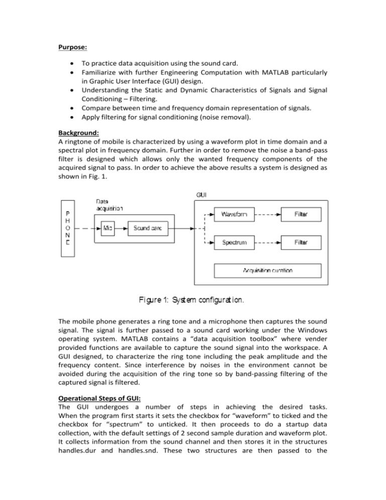
acquired signal to pass. In order to achieve the above results a system is designed as
shown in Fig. 1.
The mobile phone generates a ring tone and a microphone then captures the sound
signal. The signal is further passed to a sound card working under the Windows
operating system. MATLAB contains a “data acquisition toolbox” where vender
provided functions are available to capture the sound signal into the workspace. A
GUI designed, to characterize the ring tone including the peak amplitude and the
frequency content. Since interference by noises in the environment cannot be
avoided during the acquisition of the ring tone so by band-passing filtering of the
captured signal is filtered.
Operational Steps of GUI:
The GUI undergoes a number of steps in achieving the desired tasks.
When the program first starts it sets the checkbox for “waveform” to ticked and the
checkbox for “spectrum” to unticked. It then proceeds to do a startup data
collection, with the default settings of 2 second sample duration and waveform plot.
It collects information from the sound channel and then stores it in the structures
handles.dur and handles.snd. These two structures are then passed to the
‘plotwaveform’ function. This then completes the autonomous startup procedure.
Continuing on from this point, the GUI requires user interaction to determine its
course of action.
Waveform/Spectrum Checkbox Panel:
The user has the option to choose either a waveform plot of the results or a
spectrum graph. To determine which is created, this gui employs a panel of
checkboxes. The functions used to determine this are rather straightforward. In both
cases, the functions read the value of the checkbox (1 or 0), and then uses this to
change the values of the handles.waveform & handles.spectrum scalars within the
handles structure. It achieves this by using a series of “if statements”, if the
waveform checkbox value is 1 then handles.waveform=1 and handles.spectrum=0,
and vice versa. In order to ensure the mutual exclusivity of the waveform and
spectrum selections, the program also sets the value of the opposing checkbox to 0
when the desired checkbox is ticked, i.e. if the waveform checkbox is ticked, the
spectrum checkbox is set to 0 and becomes unticked.
Duration Drop Menu:
The user is able to select the duration that sound is recorded from the microphone
for. This is done by making a selection on a drop-down menu. The function for this
feature reads the selected value using the ‘get’ function, and then sets the scalar
value ‘handles.dur’ within the handles structure to the selected value (2,5 or 10). It
then
saves
this
value
and
the
function
finishes.
Start Button:
This function is very similar to the autonomous startup function of this program. It
first reads in the selected collection duration (handles.dur), and then collects data
from the sound channel. Once this data is collected, it then checks the value of
handles.waveform and handles.spectrum, and then passes the collected data to
either the plotwaveform function or the plotspectrum function, using a series of ‘if’
statements.
Filter button:
This function first checks to see if there is recorded sound data, by checking the
length of the snd.data vector. If there is data, it then makes use of inbuilt filtering
functions to filter the data within snd.data. Once this data is filtered, it is saved in
handles.snd.filter. Then, the program passes this information to either the filtered
waveform plot function or the filtered spectrum function, this of course is
dependent on the values of handles.waveform and handles.spectrum, with the
program checking this with ‘if’ statements, much like the start button.
Waveform Plot:
This function is straightforward for the most part, it first setups up a vector of values,
equally spaced according to the sampling rate, from 0 to the end value. It then plots
this vector against the values collected for the amplitudes of the sounds, using the
inbuilt ‘plot’ function. This appears on the axes within the GUI. In addition to this
plot, the function finds the maximum value of snd.data using “max” and then prints
this
value
in
the
title
of
the
plot.
Spectrum Plot:
This is a mostly straightforward function, as most of the procedure is done by the
inbuilt periodogram function in MATLAB. the handles.snd structure is passed into
this function, and snd.data and snd.rate are passed into the periodogram function to
create the spectrum graph. Once the function has completed this process, it then
determines the maximum power density using the inbuilt ‘max’ function. It then
prints this in the title of the plot.
Waveform Plot Filtered:
This function is nearly identical to the unfiltered waveform plot function. It first plots
the unfiltered snd.data data, in the default blue colour, using the ‘plot’ function. this
plot is then ‘held on’ and another plot is plotted over the top, that is the snd.filter
vector. This is plotted in red, so you can see the two different data series. This
function does not calculate any maximum values, as the given example does not
specify it.
Filtered Spectrum Plot:
This function is somewhat different from the unfiltered spectrum plot function, as it
was impossible to change the colour of the plot to the desired red using the
periodogram function. As thus, in this function, the periodogram function is
employed, however, it does not create a plot, but rather passes the resultant vectors
to spe.Pxx and spe.F, these values are then plotted using the plot function in such a
way that it mimics the results of the periodogram function. This is done firstly using
the snd.data vector in blue, and then the snd.filter vector is over laid in red. This
concludes the operations of the GUI, however, it is able to continue to collect and
display information indefinitely.
Theoretical Background:
A system takes an input quantity (sound signal) and transforms it into an output
quantity (waveform or spectrum) that can be observed or recorded. The shape and
form of a signal are often referred to as its waveform. The waveform contains
information about the magnitude, which indicates the size of the input quantity, and
the frequency, which indicates the way the signal changes in time. Description of the
waveform associated with a signal is useful. A signal is the physical information
about a measured variable being transmitted between a process and the
measurement system, between the stages of a measurement system, or the output
from a measurement system. Signals are classified as analog, discrete time and
digital. Digital signals are particularly useful when data acquisition and processing
are performed by using a digital computer. Signals may be characterized as either
static or dynamic. For this task digital signals are used and signal has a nondeterministic dynamic character. A dynamic signal is defined as a time-dependent
signal. A nondeterministic signal that has no discernible pattern of repetition and it
cannot be prescribed before it occurs, although certain characteristics of the signal
may be known in advance. Nondeterministic signals are generally described by their
statistical characteristics or a model signal that represents the statistics of the actual
signal.
Equations governing dynamic a periodic signals:
Figure-1: Equations representing dynamic signals
Non-deterministic variable:
Figure-2: Example of non-deterministic signal
For non- deterministic it is possible to separate a complex signal into a number of
sine and cosine functions as shown in equation below. This representation of a signal
as a series of sines and cosines is called a Fourier series. It allows essentially all
mathematical functions of practical interest to be represented by an infinite series of
sines and cosines.
Frequency Spectrum:
The Fourier transform is a complex number having a magnitude and a phase,
The magnitude of Y (f ), also called the modulus, is given by:
and the phase by:
Filter:
A filter is used to remove undesirable frequency information from a dynamic signal.
Filters can be broadly classified as being low pass, high pass, bandpass, and notch. In
this experiment task of noise removal is achieved by using band pass filter. Figure
below shows the typical design of band pass filter.
Figure-2: Filter specification
Conclusion:
In this experiment the peak amplitude, maximum power density and the
corresponding frequency of our phone’s ring tone is calculated. Ringtone of mobile
phone is classified as dynamic signal and signal has a non-deterministic dynamic
character. In order to remove the noise from the input signal ‘band-type filter’ is
used we also can attenuate other noises which are not in the frequency range of the
phone. It can be examined from the results that the change due to the filter can be
significantly seen in frequency domain graph whereas in time domain graph only
predicts that the amplitude is reduced. In spectrum plot it can be noticed that the
signal magnitude at high frequency decreases which occurs due to the fact that
microphone is insensitive to high frequencies.
Peak amplitude of the ring tone is
Dominating frequency of the ring tone is
Maximum power density of the ring tone is
Appendix:
function varargout = labweek7(varargin)
% LABWEEK7 M-file for labweek7.fig
% LABWEEK7, by itself, creates a new LABWEEK7 or raises the existing
% singleton*.
%
% H = LABWEEK7 returns the handle to a new LABWEEK7 or the handle to
% the existing singleton*.
%
% LABWEEK7('CALLBACK',hObject,eventData,handles,...) calls the local
% function named CALLBACK in LABWEEK7.M with the given input arguments.
%
% LABWEEK7('Property','Value',...) creates a new LABWEEK7 or raises the
% existing singleton*. Starting from the left, property value pairs are
% applied to the GUI before labweek7_OpeningFcn gets called. An
% unrecognized property name or invalid value makes property application
% stop. All inputs are passed to labweek7_OpeningFcn via varargin.
%
% *See GUI Options on GUIDE's Tools menu. Choose "GUI allows only one
% instance to run (singleton)".
%
% See also: GUIDE, GUIDATA, GUIHANDLES
% Edit the above text to modify the response to help labweek7
% Last Modified by GUIDE v2.5 11-Sep-2011 10:47:36
% Begin initialization code - DO NOT EDIT
gui_Singleton = 1;
gui_State = struct('gui_Name',
mfilename, ...
'gui_Singleton', gui_Singleton, ...
'gui_OpeningFcn', @labweek7_OpeningFcn, ...
'gui_OutputFcn', @labweek7_OutputFcn, ...
'gui_LayoutFcn', [] , ...
'gui_Callback', []);
if nargin && ischar(varargin{1})
gui_State.gui_Callback = str2func(varargin{1});
end
if nargout
[varargout{1:nargout}] = gui_mainfcn(gui_State, varargin{:});
else
gui_mainfcn(gui_State, varargin{:});
end
% End initialization code - DO NOT EDIT
% --- Executes just before labweek7 is made visible.
function labweek7_OpeningFcn(hObject, eventdata, handles, varargin)
% This function has no output args, see OutputFcn.
% hObject handle to figure
% eventdata reserved - to be defined in a future version of MATLAB
% handles structure with handles and user data (see GUIDATA)
% varargin command line arguments to labweek7 (see VARARGIN)
clc;%clear command window
handles.Start='';
handles.Spectrum=0;
handles.Waveform=1;
set(handles.Waveformbox,'Value',1);
set(handles.Spectrumbox,'Value',0);
set(handles.Start,'enable','off');%disable Start until end of acquistion
dur.sec=2;%default acquisition duration, dur is a structure
snd.rate=8000;%sound card sampling rate, snd is a structure
snd.AI = analoginput('winsound');%create sound object
addchannel(snd.AI,1);%1 sound channel
set(snd.AI,'SampleRate',snd.rate);%setup sound card
set(snd.AI,'SamplesPerTrigger',dur.sec*snd.rate);%setup
start(snd.AI); wait(snd.AI,dur.sec+0.5);%start acquisition
snd.data=getdata(snd.AI);%get data from sound card
snd.data=OffsetData(snd.data);%offset data to its mean value
delete(snd.AI); clear snd.AI;%finished acquistion
PlotWaveform(dur,snd);%plot the default waveform
set(handles.Start,'enable','on');%enable Start pushbutton
handles.snd=snd; handles.dur=dur;%store data
% Choose default command line output for labweek7
handles.output = hObject;
% Update handles structure
guidata(hObject, handles);
% UIWAIT makes labweek7 wait for user response (see UIRESUME)
% uiwait(handles.figure1);
% --- Outputs from this function are returned to the command line.
function varargout = labweek7_OutputFcn(hObject, eventdata, handles)
% varargout cell array for returning output args (see VARARGOUT);
% hObject handle to figure
% eventdata reserved - to be defined in a future version of MATLAB
% handles structure with handles and user data (see GUIDATA)
% Get default command line output from handles structure
varargout{1} = handles.output;
%SPECTRUM CHECKBOX
% --- Executes on button press in Spectrumbox.
function Spectrumbox_Callback(hObject, eventdata, handles)
% hObject handle to Spectrumbox (see GCBO)
% eventdata reserved - to be defined in a future version of MATLAB
% handles structure with handles and user data (see GUIDATA)
val = get(hObject,'Value');
if val == 1;
set(handles.Waveformbox,'Value',0);
handles.Waveform=0;
handles.Spectrum=1;
end;
if val == 0;
handles.Spectrum=0;
handles.Waveform=1;
end;
guidata(hObject, handles);
% Hint: get(hObject,'Value') returns toggle state of Spectrumbox
% --- Executes on selection change in Durationselect.
function Durationselect_Callback(hObject, eventdata, handles)
% hObject handle to Durationselect (see GCBO)
% eventdata reserved - to be defined in a future version of MATLAB
% handles structure with handles and user data (see GUIDATA)
% Determine the selected data set.
str = get(hObject, 'String');
val = get(hObject,'Value');
% Set current data to the selected data set.
switch str{val};
case '2'
handles.dur.sec=2;
case '5'
handles.dur.sec=5;
case '10'
handles.dur.sec=10;
end
% Update handles structure
guidata(hObject, handles);
% Hints: contents = cellstr(get(hObject,'String')) returns Durationselect contents as
cell array
%
contents{get(hObject,'Value')} returns selected item from Durationselect
% --- Executes during object creation, after setting all properties.
function Durationselect_CreateFcn(hObject, eventdata, handles)
% hObject handle to Durationselect (see GCBO)
% eventdata reserved - to be defined in a future version of MATLAB
% handles empty - handles not created until after all CreateFcns called
% Hint: popupmenu controls usually have a white background on Windows.
%
See ISPC and COMPUTER.
if ispc && isequal(get(hObject,'BackgroundColor'),
get(0,'defaultUicontrolBackgroundColor'))
set(hObject,'BackgroundColor','white');
end
%START BUTTON
% --- Executes on button press in Startbutton.
function Startbutton_Callback(hObject, eventdata, handles)
% hObject handle to Startbutton (see GCBO)
% eventdata reserved - to be defined in a future version of MATLAB
% handles structure with handles and user data (see GUIDATA)
%handles.Waveform
snd=handles.snd;
dur=handles.dur;
snd.AI = analoginput('winsound');%create sound object
addchannel(snd.AI,1);%1 sound channel
set(snd.AI,'SampleRate',snd.rate);%setup sound card
set(snd.AI,'SamplesPerTrigger',dur.sec*snd.rate);%setup
start(snd.AI); wait(snd.AI,dur.sec+0.5);%start acquisition
snd.data=getdata(snd.AI);%get data from sound card
snd.data=OffsetData(snd.data);%offset data to its mean value
delete(snd.AI); clear snd.AI;%finished acquistion
handles.snd=snd;
handles.dur=dur;
if handles.Waveform == 1
PlotWaveform(handles.dur,handles.snd);
end
if handles.Spectrum == 1
PlotSpectrum(handles.snd);
end
guidata(hObject, handles);
% --- Executes on button press in Filterbutton.
function Filterbutton_Callback(hObject, eventdata, handles)
% hObject handle to Filterbutton (see GCBO)
% eventdata reserved - to be defined in a future version of MATLAB
% handles structure with handles and user data (see GUIDATA)
if length(handles.snd.data)>0,
dur=handles.dur; snd=handles.snd; Fs=snd.rate;
A_stop1 = 30; % Attenuation in the first stopband = 30 dB
F_stop1 = 800; % Edge of the stopband = 800 Hz
F_pass1 = 1000; % Edge of the passband = 1000 Hz
F_pass2 = 2000; % Closing edge of the passband = 2000 Hz
F_stop2 = 2200; % Edge of the second stopband = 2200 Hz
A_stop2 = 30; % Attenuation in the second stopband = 30 dB
A_pass = 1; % Allowed ripple in the passband = 1 dB
BandPassSpecObj = ...
fdesign.bandpass('Fst1,Fp1,Fp2,Fst2,Ast1,Ap,Ast2',...
F_stop1,F_pass1,F_pass2,F_stop2,A_stop1,A_pass,A_stop2,Fs);
BandPassFilt = design(BandPassSpecObj, 'butter');
dur.time=1/snd.rate:1/snd.rate:dur.sec;
z=find(isnan(snd.data)); snd.data(z)=[]; dur.time(z)=[];
snd.filter=filter (BandPassFilt,snd.data);
% handles.Waveform
% handles.Spectrum
if handles.Waveform==1,
PlotWaveformFiltered(dur,snd);
end;
if handles.Spectrum==1,
PlotSpectrumFiltered(snd);
end;
end
guidata(hObject, handles);
%WAVEFORM CHECKBOX
% --- Executes on button press in Waveformbox.
function Waveformbox_Callback(hObject, eventdata, handles)
% hObject handle to Waveformbox (see GCBO)
% eventdata reserved - to be defined in a future version of MATLAB
% handles structure with handles and user data (see GUIDATA)
val = get(hObject,'Value');
if val == 1
set(handles.Spectrumbox,'Value',0);
handles.Waveform=1;
handles.Spectrum=0;
end;
if val == 0
handles.Spectrum=1;
handles.Waveform=0;
end;
% Hint: get(hObject,'Value') returns toggle state of Waveformbox
guidata(hObject, handles);
%data offset function
function [data]=OffsetData(data)
data=data-mean(data);
return;
%plot waveform filtered
function []=PlotWaveformFiltered(dur,snd)
cla;
plot(dur.time,snd.data,'b'); grid on; hold on;
plot(dur.time,snd.filter,'r'); hold off;
title('Filtered Signal');
xlabel('Time(sec)');
ylabel('Amplitude (volt)');
return;
function []=PlotSpectrum(snd)
periodogram(snd.data,[],2048,snd.rate);
[spe.Pxx,spe.F]=periodogram(snd.data,[],2048,snd.rate);
[mx,ix]=max(spe.Pxx); logmx=10*log10(mx);
title(sprintf('Max power density=%6.3f at %04.0fHz',logmx,spe.F(ix)),...
'color','r');
mlogmx=mean(10*log10(spe.Pxx)); dmx=abs(mlogmx)/2;
ax=axis; axis([ax(1:2) mlogmx-dmx mlogmx+dmx]);
return;
function [] = PlotWaveform(dur,snd)
dur.time=1/snd.rate:1/snd.rate:dur.sec;
plot(dur.time,snd.data);grid on;
title(sprintf('Peak Magnitude= %1.3f V',max(snd.data)));
xlabel('Time(sec)');
ylabel('Amplitude (volt)');
return;
function []=PlotSpectrumFiltered(snd)
%unfiltered plot
%periodogram(snd.data,[],2048,snd.rate);
[spe.Pxx,spe.F]=periodogram(snd.data,[],2048,snd.rate);
[mx,ix]=max(spe.Pxx); logmx=10*log10(mx);
mlogmx=mean(10*log10(spe.Pxx)); dmx=abs(mlogmx)/2;
ax=axis; axis([ax(1:2) mlogmx-dmx mlogmx+dmx]);
spe.Pxx = 10 * log10(spe.Pxx);
plot(spe.F/1000,spe.Pxx);grid on;hold on;
% filtered plot
%periodogram(snd.filter,[],2048,snd.rate);
[spe.Pxx,spe.F]=periodogram(snd.filter,[],2048,snd.rate);
[mx,ix]=max(spe.Pxx); logmx=10*log10(mx);
title('Filtered Signal Spectrum')
mlogmx=mean(10*log10(spe.Pxx)); dmx=abs(mlogmx)/2;
ax=axis; axis([ax(1:2) mlogmx-dmx mlogmx+dmx]);
spe.Pxx = 10 *log10(spe.Pxx);
plot(spe.F/1000,spe.Pxx,'r');
xlabel('Frequency(kHz)');
ylabel('Power Density(dB/kHz)');
hold off;
return;