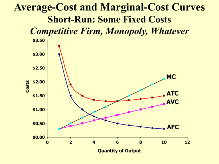
Average-Cost and Marginal-Cost Curves
Short-Run: Some Fixed Costs
Competitive Firm, Monopoly, Whatever
$3.50
$3.00
Costs
$2.50
MC
$2.00
ATC
AVC
$1.50
$1.00
$0.50
$0.00
AFC
0
2
4
6
8
Quantity of Output
10
12
Competitive Industry
Supply and Demand
Price
Supply
$3.00
Equilibrium
2.50
2.00
1.50
1.00
Demand
0.50
0
1 2 3 4 5 6 7 8 9 10 11 12
Quantity
The Competitive Firm’s Short-Run Supply Curve:
(The Competitive Firm is a Price-Taker)
Produce where MC = MR = Price > AVC
Costs
Firm’s short-run
supply curve.
If P > ATC,
keep producing
at a profit.
If P > AVC,
keep producing
in the short run.
MC
ATC
AVC
If P < AVC,
shut down.
0
Quantity
The Short Run: Market Supply with a
Fixed Number of Firms...
(a) Individual Firm Supply
Price
(b) Market Supply
Price
Supply
MC
$2.00
$2.00
1.00
1.00
0
100
200
Quantity
(firm)
0
100,000 200,000 Quantity
(market)
Industry Supply: Some Examples
1. 50 firms, each with TC(x) = 2x + .01 x2
•
•
Each firm’s supply
Industry supply
2. 50 firms with TC(x) = 2x + .01 x2
and 50 firms with TC(x) = 3x + .005 x2
•
•
Each firm’s supply
Industry supply
3. 50 firms with TC(x) = 100 + 2x + .01 x2, x > 0 ;
but TC(0) = 0, i.e., avoidable fixed cost
•
•
Each firm’s supply
Industry supply
Competitive Firm’s Supply Curve
Long Run: No Fixed Costs
Costs
MC = Long-run S
Firm enters
if P > ATC
ATC
Firm exits
if P < ATC
0
Quantity
The Long Run: Market Supply with
Entry and Exit...
(a) Firm’s Zero-Profit Condition
Price
(b) Market Supply
Price
MC
ATC
P=
minimum
Supply
ATC
0
Quantity
(firm)
0
Quantity
(market)
Response to Increase in Demand
Short - Run , Medium - Run, Long - Run
Initial equilibrium: existing firms operating at
efficient scale and earning zero profit
• Short – run: fixed number of existing firms
– Price rises each firm expands output along its MC
curve MC = Price > AC PROFITS
• Intermediate – run: additional firms enter
– Industry supply shifts outward Price declines
Reduced profits
• Long – run: additional firms continue to enter,
industry supply continues to shift increase, and price
continues to drop
Return to zero profit equilibrium
The Long Run: Competitive Market Supply
Is long – run supply truly horizontal (flat)?
Are long – run profits truly zero?
• All firms are not created equal … some are
endowed with lower costs
– More and less fertile land Rents
– Better and worse management Quasi – rents
As less and less efficient firms enter, industry supply
curve slopes upward
• Industry expansion higher input prices
higher costs for all firms
As industry expands, each firm’s minimum cost
increases industry supply curve slopes upward
Monopolistic Competition: Many Firms
with Differentiated Products
Short-Run: Firm Makes a Profit
Price
Price
Average
total cost
MC
ATC
Demand
Profit
MR
0
Profitmaximizing quantity
Quantity
Price
A Monopolistic Competitor
in the Long Run…P > MC
… but Zero Profit
MC
ATC
P=ATC
MR
0
Profit-maximizing
quantity
Demand
Quantity
Consumer Surplus and Producer Surplus:
Benefits they get from trading in the market
Price
A
D
Equilibrium
price
Supply
Consumer
surplus
E
Producer
surplus
B
Demand
C
0
Equilibrium
quantity
Quantity
Price And Consumer Surplus...
Copyright © 2001 by Harcourt, Inc. All rights reserved
Consumers benefit from price < what they’re
willing to pay, whether they face competitive firm
or monopolist
Price
A
P1
P2
Initial
consumer
surplus
B
D
Additional
consumer
surplus to
initial
consumers
0
Consumer
surplus to “new”
consumers
C
E
F
Demand
Q1
Q2
Quantity
How Price Affects Producer Surplus...
Price
Supply
Additional producer
surplus to initial
producers
P2 D
P1 B
Initial
Producer
surplus
E
F
C
Producer surplus
to new producers
A
0
Q1
Q2
Quantity
Static Efficiency of Competitive Market
Equilibrium
Price
Supply
Value
to
buyers
Cost
to
sellers
Cost
to
sellers
0
Value
to
buyers
Demand
Equilibrium
quantity
Value to buyers is greater
than cost to sellers.
Value to buyers is less
than cost to sellers.
Quantity
Insights About Market Outcomes
Free markets allocate the supply of goods to the
buyers who value them most highly.
With money-left-over utility function,
MUx/px = 1 or MUx= px same for all buyers
Free markets allocate the demand for goods to
the sellers who produce them at least cost
MCx= px same for all sellers = px = MUx
Free markets produce the quantity of goods that
maximizes the sum of consumer and producer
surplus.
But promise of monopoly profits drives innovation
The Tax Wedge and Deadweight Loss
Price
Consumer Surplus
Supply
Price Paid
Tax
Tax
Revenue
Price Rec’d
Producer Surplus
Demand
0
Quantity
