Appendix 4A
Problem 4A-1 (20 minutes)
1.
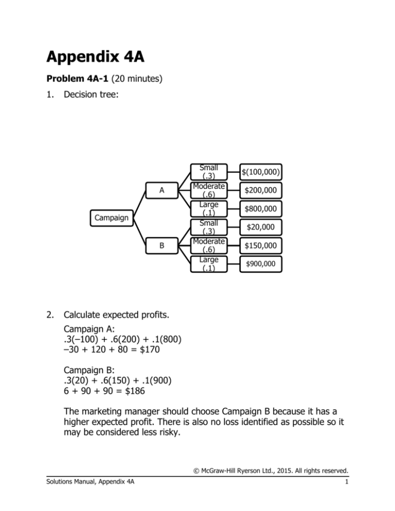
Decision tree:
A
Campaign
B
2.
Small
(.3)
Moderate
(.6)
Large
(.1)
Small
(.3)
Moderate
(.6)
Large
(.1)
$(100,000)
$200,000
$800,000
$20,000
$150,000
$900,000
Calculate expected profits.
Campaign A:
.3(–100) + .6(200) + .1(800)
–30 + 120 + 80 = $170
Campaign B:
.3(20) + .6(150) + .1(900)
6 + 90 + 90 = $186
The marketing manager should choose Campaign B because it has a
higher expected profit. There is also no loss identified as possible so it
may be considered less risky.
© McGraw-Hill Ryerson Ltd., 2015. All rights reserved.
Solutions Manual, Appendix 4A
1
Problem 4A-2 (20 minutes)
(a) Decision Tree
Make
Options
Buy
High
(.3)
Medium
(.4)
Low
(.3)
High
(.3)
Medium
(.4)
Low
(.3)
$150,000
$90,000
$(30,000)
$105,000
$90,000
$25,000
(b) For “make” alternative:
Expected profits = (.3 × 150) + (.4 × 90) + (.3 × -30)
= 45 + 36 – 9
= 72
= $72,000
For “buy” alternative:
Expected profits = (.3 × 105) + (.4 × 90) + (.3 × 25)
= 31.5 + 36 + 7.5
= 75
= $75,000
The company should buy the subassembly because it has a higher
expected operating profit. There is also no loss identified which indicates a
lower risk.
(CGA-Canada Solution, adapted)
© McGraw-Hill Ryerson, 2015. All rights reserved.
2
Managerial Accounting, 10th Canadian Edition
Problem 4A-3 (20 minutes)
IF Win
Proposals Revenue
A
$1,000,000
B
1,000,000
IF Lose
A
B
0
0
Costs
$300,000
100,000
300,000
100,000
Net
Tax 30%
$700,000 $210,000
900,000
270,000
(300,000)
(100,000)
Win (.6)
$490,000
Lose (.4)
$(210,000)
Win (.2)
$630,000
Lose (.8)
$(70,000)
90,000
30,000
After Tax
$ 490,000
630,000
(210,000)
(70,000)
A
Proposals
B
Expected profits:
Proposal A: ($490,000 x .6) + (-$210,000 x .4)
$294,000 -$84,000 = $210,000
Proposal B: ($630,000 x .2) + (-$70,000 x .8)
$126,000 -$56,000 = $70,000
Since Proposal A has the higher expected value, it should be submitted to
the city.
(SMAC, adapted)
© McGraw-Hill Ryerson Ltd., 2015. All rights reserved.
Solutions Manual, Appendix 4A
3
Case 4A-4 (45 minutes)
Unit Contribution Margin Analysis
Expected contribution margins per unit at the three suggested selling
prices are as follows:
Selling price ...........................................
Variable costs ($2,800,000 ÷ 350,000) ....
Contribution margin/unit .........................
$24.00
8.00
$16.00
$27.00
8.00
$19.00
$31.50
8.00
$23.50
Expected Value Analysis
Market Research Data
Volume
Expected
Probability Volume
Selling price = $24.00
500,000
.20
400,000
.50
300,000
.30
1.00
Unit
CM
Total
Expected
Contribution
Margin
Ranking
100,000
200,000
90,000
390,000
$16.00
$6,240,000
2
100,000
157,500
75,000
332,500
$19.00
$6,317,500
1
90,000
125,000
40,000
255,000
$23.50
$5,992,500
3
Selling price = $27.00
400,000
350,000
250,000
.25
.45
.30
1.00
Selling price = $31.50
300,000
250,000
200,000
.30
.50
.20
1.00
© McGraw-Hill Ryerson, 2015. All rights reserved.
4
Managerial Accounting, 10th Canadian Edition
Case 4A-4 (continued)
President’s Data
Volume
Expected
Probability Volume
Unit
CM
Total
Expected
Contribution
Margin
Ranking
Selling price = $24.00
500,000
400,000
300,000
.10
.50
.40
1.00
50,000
200,000
120,000
370,000
$16.00
$5,920,000
3
80,000
140,000
100,000
320,000
$19.00
$6,080,000
2
120,000
125,000
20,000
265,000
$23.50
$6,227,500
1
Selling price = $27.00
400,000
350,000
250,000
.20
.40
.40
1.00
Selling price = $31.50
300,000
250,000
200,000
.40
.50
.10
1.00
(Note, in all cases for both market research and president’s data, CM is
high enough to cover fixed overhead.)
From the preceding analysis, we arrive at two different optimum solutions.
Using the market research data, setting the selling price slightly below the
competition at $27.00 would yield the highest expected contribution.
However, the president’s data indicate that it would be best to set the price
above that of the competition, representing full cost plus 100 percent.
Because the rankings are significantly different, we must examine other
factors to determine the best pricing strategy.
© McGraw-Hill Ryerson Ltd., 2015. All rights reserved.
Solutions Manual, Appendix 4A
5
Case 4A-4 (continued)
Factors to Consider
1.
Accuracy of data—One must examine the underlying assumptions on
which the data are based. Although the market research data are based
on “extensive” market testing, the manner in which the testing was
conducted, the composition of the test market, the design of the test, etc.,
must be examined for their appropriateness. Key factors such as quality
of product, warranties, etc., may exist which may not have been
considered in the market test. Since the president has past experience to
draw from and also has knowledge of factors other than price, his data
may be more accurate. On the other hand, the president could be
imposing personal biases and “wishful thinking” which could render his
data to be overly optimistic.
2.
Product life cycle and elasticity of demand—The market research data
indicate that demand for this product is fairly elastic and the president’s
data reflect a slightly less elastic demand. Both sets of data assume that
demand would remain constant over a five-year period. This is highly
unlikely. Since this is a relatively new product on the market, it is in the
infant stage of its life cycle. Generally, appliance-type products would
start with relatively few competitors and fairly inelastic demand.
Therefore, a high-price/low-volume (skimming) strategy would be
appropriate. Then, as the market begins to accept the product, volumes
would increase as prices decline to a fairly stable level—also, at this
point, more competitors would enter similar products into the market.
Finally, as new substitute products enter the market, volumes and prices
would drop. The volumes indicated in both the market research and
president’s data would be useful only for the short term. The product
cycle would drastically affect the price/volume behaviour in the long term.
The fact that the product is now in the infant stage would lend some
support to the president’s data for the short term. The market research
data may possibly represent a long-term averaging which may better
reflect market behaviour two or three years from now.
© McGraw-Hill Ryerson, 2015. All rights reserved.
6
Managerial Accounting, 10th Canadian Edition
Case 4A-4 (continued)
3.
Reactions of competitors—One must examine whether BL has historically
been a price leader or price follower. If it is generally a price leader, it may
be safe to assume that competitors will follow whatever price BL decides
to set, which may drastically influence the projected data. On the other
hand, if BL is normally a price follower, competitors would probably have
no reaction to BL pricing at a skimming price of $31.50.
However, if BL enters the market with a price of $27.00 or $24.00,
competitors may react by undercutting BL, and starting a price war,
especially if the competitors have cost structures similar to BL (i.e.,
relatively low variable costs resulting in high contribution margins).
4.
Nature of the competitive market—BL must investigate whether the
cordless curling irons sold by the competition are of better, worse, or
same quality as BL’s iron and whether they offer special features or
different warranties from those of BL. If BL offers better features,
quality, and services, customers will be willing to pay a higher price.
5.
Past relations with customers and competitive advantages—BL’s past
relations and reputation with its customers would have a great impact on
the success of the new product. Customers may be willing to pay more
for BL’s product if, in the past, factors such as product and service
quality, warranties, credit terms, flexibility, effectiveness of advertising,
brand-name loyalties, etc., have resulted in customers favouring its
products. Conversely, customer relations with competitors would also
have an impact on the demand that BL can expect for its product. BL
must consider how customers would perceive a low, middle, or high price
(i.e., if priced at $24.00, would customers think the product is inferior or
that it is a better buy?)
6.
Opportunity costs and production constraints—BL currently has capacity
to produce 500,000 units per year. Assuming that the maximum expected
annual demand over the next 5 years is 500,000 units, we need only be
concerned with the opportunity costs of producing cordless curling irons
versus utilizing the same capacity by producing some other product. BL
must examine whether there are more profitable options for utilizing
this capacity in both the short term and the long term. Also, BL should
consider if it can profitably utilize the excess capacity if it adopts a highprice/low-volume pricing strategy.
© McGraw-Hill Ryerson Ltd., 2015. All rights reserved.
Solutions Manual, Appendix 4A
7
Case 4A-4 (continued)
7.
Sensitivity of the volume projections—The sensitivity of the volume
projections should be examined to determine the safety margin in the
case that the sales projections do not materialize.
Price
$24.00
27.00
31.50
CM/Unit
$16.00
19.00
23.50
Fixed Costs
$2,712,500
2,712,500
2,712,500
Break-Even
Volume (Units)
169,532
142,764
115,426
From the analysis, it can be seen that there is a large margin of safety at
each of the prices. Volumes can be considerably lower than the lowest
projected volumes before BL would experience losses.
8.
BL’s cost structure—The unit variable cost of $8.00 per unit is based on a
volume of 350,000 units and the cost projection at this volume is likely
based on engineered standards and production of prototypes. Actual unit
variable costs may be somewhat higher at annual volumes less than
350,000 units or may be somewhat lower at annual volumes greater than
350,000 units. This is due to economies of scale and the learning curve. It
would be reasonable to expect that unit variable costs would decrease
over time as a result of the learning curve effect which would give BL
additional pricing flexibility in the latter years of the product life cycle.
9.
Alternative pricing policies—Variable-cost pricing generally determines
the “floor” price that a company requires to cover its direct variable
costs. This strategy is easy to develop; it offers easy insights into
cost/volume/profit relationships and into short-term pricing decisions.
Another advantage is that variable costs tend to be reliable and fairly
accurate. One drawback is that it may lead to under-pricing because it
does not consider fixed costs.
© McGraw-Hill Ryerson, 2015. All rights reserved.
8
Managerial Accounting, 10th Canadian Edition
Case 4A-4 (continued)
Full-cost pricing considers all costs in the pricing decision. However,
determination of full costs requires an allocation of joint costs to
products. Allocation bases are arbitrary, and very different cost
structures can result depending on the allocation base. Also, this pricing
strategy is circular. When products are price elastic, price determines
volume and, in full-cost pricing, volume determines unit cost, and unit
cost determines price. For example, using the president’s data, a $31.50
price for the new curling iron would result in an expected volume of say
265,000 units. Full cost per unit, therefore, would be $8.00 + $10.24 =
$18.24. Full cost + 100 percent equals a selling price of $36.48. At this
price, the expected volumes would certainly drop.
Other pricing policies that could be considered in the short term are
market pricing, target gross margin, return on assets employed,
standard costs plus, and pricing to achieve some target market share.
RECOMMENDATION
Assuming that the president’s data took into account some non-price
competitive advantages which the market research data did not consider, I
would recommend setting the price initially at $31.50 and consider lowering
the price after one or two years once the product life has matured a bit and
any economies of scale have been achieved. This strategy would allow BL to
take advantage of its idle capacity for other opportunities. Consideration
should be given to supporting the product introduction with an extensive
advertising and promotional campaign.
Another valid recommendation could be to set the price initially at $27.00.
This strategy would undercut the competition but would likely not cause a
price war. With this strategy, BL would maintain its quality image by
emphasizing to customers that it is letting them benefit from BL’s production
efficiency and not allowing the competitors to skim the market.
(SMAC Solution, adapted)
© McGraw-Hill Ryerson Ltd., 2015. All rights reserved.
Solutions Manual, Appendix 4A
9
